Welcome to the blog

Posts

My thoughts and ideas

Introduction to R Markdown | Griffith Lab

Genomic Visualization and Interpretations

Introduction to R Markdown

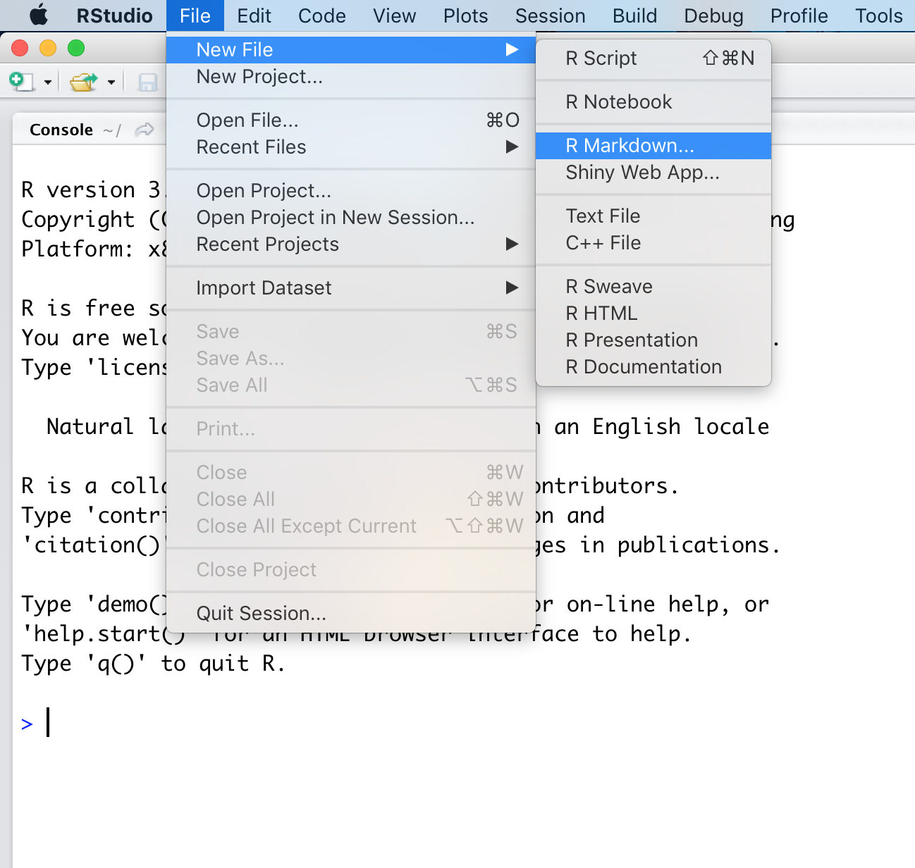
A useful feature within the R ecosystem is R Markdown. R Markdown (or .Rmd) files allow a user to intersperse notes with code providing a useful framework for sharing scientific reports in a transparent and easily reproduceable way. They combine both markdown syntax for styling notes and Rscripts for running code and producing figures. Reports can be output in a variety of file formats including HTML documents, PDF documents, and even presentation slides.

Installing R Markdown

  • To start let’s make a simple R Markdown file with Rstudio, you will need to install the R Markdown package from cran.
    # install R Markdown
    install.packages("rmarkdown")
    

R Markdown basics

  • Once R Markdown has been installed we can select File -> New File -> R Markdown to create an intial rmarkdown template.
  • Rstudio will ask you to choose an output format, and to add a title and author, for now we will just use the default HTML format however this can be changed at any time within the Rmarkdown template.
  • Go ahead and select okay when you have added your name and a title.

Rstudio should now have made a template for us, let’s go over a few introductory topics related to this template. At the top of the file you will see what looks like a YAML header denoted by ---. This is where the defaults for building the file are set.

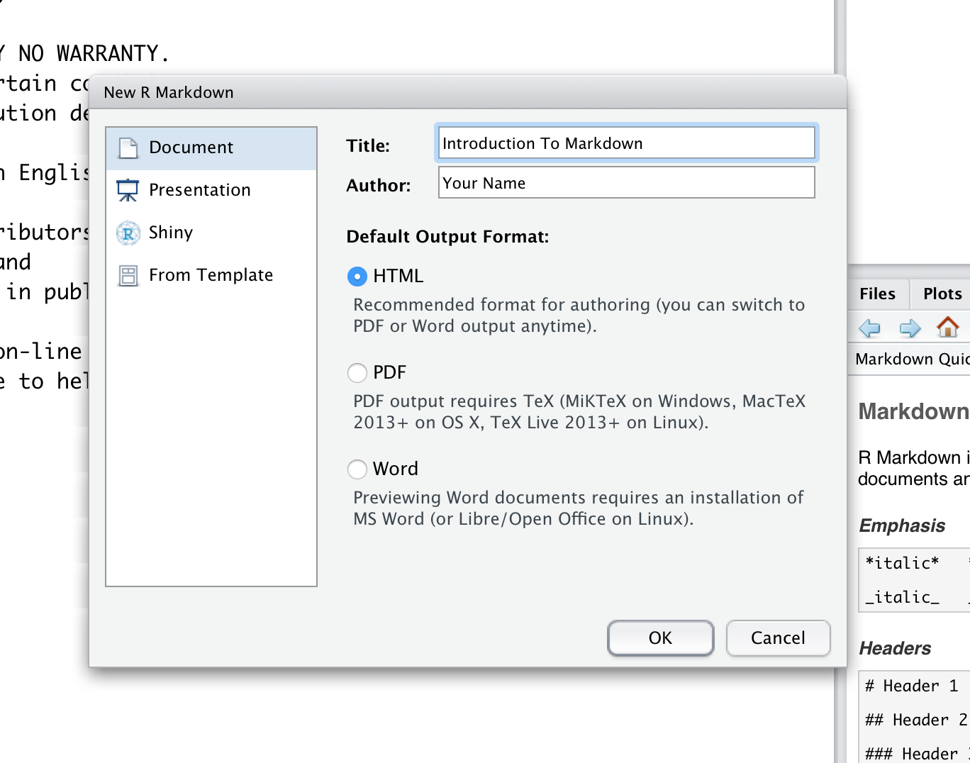
You will notice that R Markdown has pre-populated some fields based on what we supplied when we initalized the markdown template. You can output the R Markdown (.Rmd) document using the Knit button in the top left hand corner of RStudio. This is the same as calling the function render() which takes the path to the R Markdown file as input. This file should end in a .Rmd extension to denote it as an rmarkdown file, though Rstudio will take care of this for you the first time you hit Knit.

Rstudio also has a convenient way to insert code using the insert button to the right. You might notice that not only does rmarkdown support R, but also bash, python and a few other languages as well. Though in order to work, these languages will need to be installed before using Knit.

  • Go ahead and hit the Knit button just to see what an R Markdown output looks like with the default example text. If you are working with the default HTML option the result will load in a new RStudio window with the option to open it in your usual web browser.

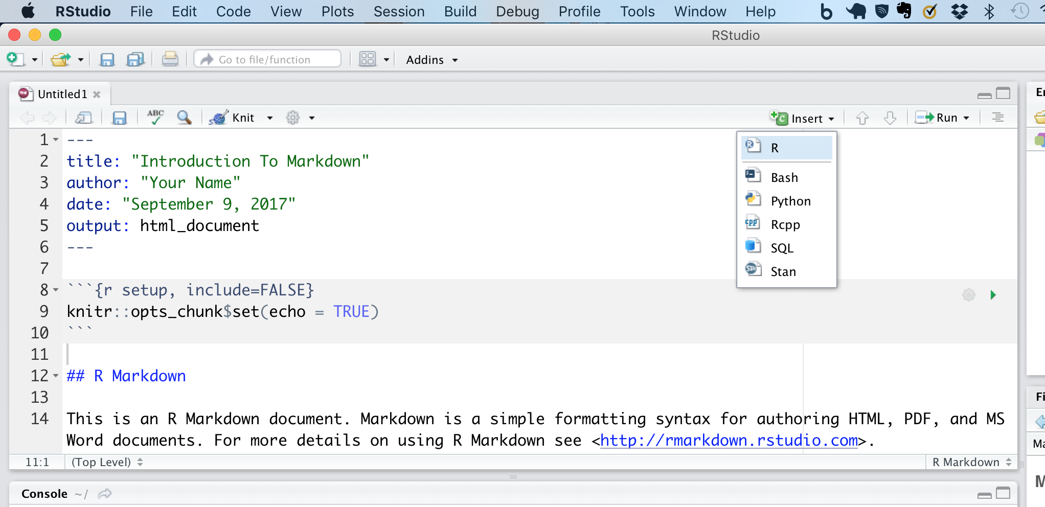
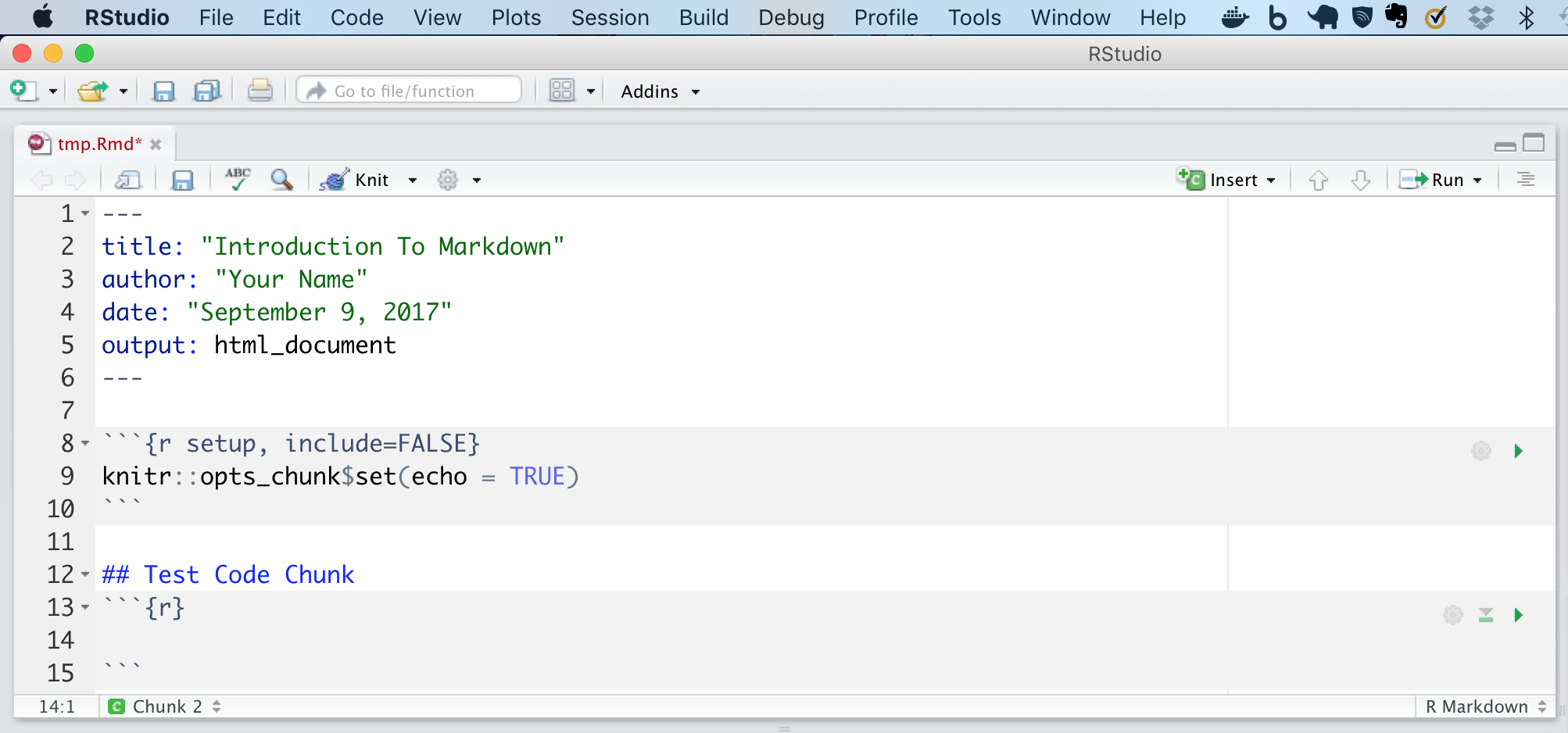
Note: you use “include=FALSE to have the chunk evaluated, but neither the code nor its output displayed.

Creating a report

Now that we’ve gone over the basics of R Markdown let’s create a real (but simple) report. First, you’ll need to download the Folicular Lymphoma data set we used in the previous ggplot2 section. Go ahead and download that dataset from http://www.genomedata.org/gen-viz-workshop/intro_to_ggplot2/ggplot2ExampleData.tsv if you don’t have it.

R Markdown documents combine text and code, the text portion of these documents use a lightweight text markup language known as markdown. This allows text to be displayed in a stylistic way on the web without having to write HTML or other web code. We won’t go over all of markdowns features however it will be good to familiarize yourself with this style.

A cheatsheet for the markdown flavor that R Markdown uses can be found by going to help -> Cheatsheets -> R Markdown Cheatsheets.

As we have mentioned you can insert a code chunk using the insert button on the top right. For example as shown below when selecting insert -> R, we get a code chunk formatted for R. However you can also add parameters to this code chunk to alter it’s default behavior. A full list of these parameters is available here.

Exercises

We have created a preliminary rmarkdown file you can download here.

Fill in this document to make it more complete, and then knit it together. The steps you should follow are outlined right in this R Markdown document. You can open this file in RStudio by going to File -> Open File. An R Markdown reference is available here.

Get a hint!

Look at the R Markdown reference guide mentioned above or the cheatsheets in Rstudio.

Answer

Here is a more complete .Rmd file.

Introduction to shiny | Griffith Lab

Genomic Visualization and Interpretations

Introduction to shiny

Interactive graphics is an emerging area within R. There are many libraries available to make interactive visualizations, however most of these libraries are still quite new. In this sub-module we will give a brief overview of shiny, a web application framework within R for building interactive web pages. Using shiny we will build a simple application to display our data using reactive data sets and ggplot.

Install shiny

The shiny package is available on cran and is fairly easy to install using install.packages(). Go ahead and install and load the package. The package comes with 11 example apps that can be viewed using the runExample() function, we will be building our own app from scratch, but feel free to try out a few of these examples to get a feel for what shiny can do. Shiny also provides a nice gallery of example applications and even a genomics example plotting cancer genomics data in a circos-style application.

# install and load shiny
install.packages("shiny")
library(shiny)

# list the built in shiny app examples
runExample()

# run one of these examples in Rstudio
runExample("06_tabsets")

What shiny is actually doing here is converting the R code to html pages and serving those on a random port using the ip address 127.0.0.1 which is localhost on most computers. In simplified terms these html pages are simply being hosted by your own computer. If you are in Rstudio your web application should have been opened automatically, however you can also view these with any modern web browser by going to the web address listed after calling runExample(). It should look something like this: http://127.0.0.1:4379.

After checking it out, use the escape key to stop the shiny app.

Structure of a shiny app

The basic code to run any shiny app is split into two parts: the server (e.g., server.R) and user interface (e.g., ui.R). The server script is the back end of our shiny web app and contains the instructions to build the app. The user interface script is the front end and is essentially what a user views and interacts with. Both of these files should be in the same directory for the app to work properly.

Go ahead and make a folder for our shiny app called “testApp”.

Next create the following two scripts there: ui.R and server.R. This is the bare minimum for a shiny app and will generate an empty web application.

# load shiny library
library(shiny)

# set up front end
shinyUI(fluidPage(
))
# load shiny library
library(shiny)

# set up back end
shinyServer(function(input, output) {
})

To view/test your app simply type the runApp(port=7777) command in your R/Rstudio terminal. For convenience in this tutorial, we have selected a specific port instead of letting shiny choose one randomly.

Make sure that your current working directory in R is set to the top level of “testApp” where you put server.R and ui.R.

You can use getwd() and setwd() to print and set this respectively.

Example:

getwd()
setwd("/Users/mgriffit/Desktop/testApp")
getwd()
runApp(port=7777)

If successful, Rstudio will display a new window with your application running. Alternatively you can view your app in a web browser at http://127.0.0.1:7777. So far, all you should see is an empty page.

Loading data into the shiny back end (server)

Now that we’ve got a basic frame work up let’s go ahead and load some data and answer a few questions. The data we will use is supplemental table 6 from the paper “Comprehensive genomic analysis reveals FLT3 activation and a therapeutic strategy for a patient with relapsed adult B-lymphoblastic leukemia.”. The data contains variant allele frequency (VAF) values from a targeted capture sequencing study of an adult AML patient with 11 samples of various cell populations and timepoints.

You can download the table here. For simplicity, make a “data” directory in your app and place the data file there.

We can load this data into shiny as you would any other data in R. Just be sure to do this in the server.R script and place the code within the unamed function. Add the following to your server.R script to make the data available within the shiny server.

# load shiny library
library(shiny)

# set up back end
shinyServer(function(input, output) {
    # load the data
    amlData <- read.delim("data/shinyExampleData.tsv")
})

Sending output to the shiny front end (UI)

Now that we have data let’s make a quick plot showing the distribution of VAF for the normal skin sample (Skin_d42_I_vaf) in comparison to the initial tumor marrow core sample (MC_d0_clot_A_vaf) and send it to the app’s user interface.

We’ll need to first create the plot on the back end (i.e. server.R). We can use any graphics library for this, but here we use ggplot2.

In order to be compatible with the shiny UI we call a Render function, in this case renderPlot() which takes an expression (i.e. set of instructions) and produces a plot. The curly braces in renderPlot() just contain the expression used to create the plot and are useful if the expression takes up more than one line. The renderPlot() will do some minimal pre-processing of the object returned in the expression and store it to the list-like “output” object.

Notice that in the ui.R file we have added a mainPanel() which, as it sounds, is instructing the app to create a main panel on the user interface. Now that we have somewhere to display our plot we can link what was created on the back end to the front end. This is done with the Output family of functions, in this case our output is a plot generated by renderPlot() and is stored in the list like output object as “scatterplot” created in the server.R file.

We use plotOutput() to provide this link to the front end and give the output ID, which is just the name of the object stored in the output-like list.

Note that when providing this link the type of object created with a Render function must correspond to the Output function, in this example we use renderPlot() and plotOutput() but other functions exist for other data types such as renderText() and textOuput().

# load shiny library
library(shiny)

# set up front end
shinyUI(fluidPage(
    mainPanel(plotOutput("scatterPlot"))
))
# load shiny library
library(shiny)

# set up back end
shinyServer(function(input, output) {
    # load the data
    amlData <- read.delim("data/shinyExampleData.tsv")

    # construct a plot to show the data
    library(ggplot2)
    output$scatterPlot <- renderPlot({
        p1 <- ggplot(amlData, aes(x=Skin_d42_I_vaf, y=MC_d0_clot_A_vaf)) + geom_point()
        p1
    })
})

Once again, to view/test your app simply type the runApp(port=7777) command in your R/Rstudio terminal and go to http://127.0.0.1:7777.

This should happen automatically from Rstudio. If your previous app is still running you may need to stop and restart it and/or refresh your browser. You should now see a ggplot graphic in your browser (see below). But, so far, nothing is interactive about this plot. We will allow some basic user input and interactivity in the next section.

Now using what we’ve learned so far try to add some text to are web app by passing it from the back end to the front end.

Get a hint!

Look at the help for textInput textOutput() and renderText renderText()

Solution

These files contain a correct answer: ui.R, server.R

When you’ve completed the above exercise try and answer a few of the questions below.

Why would you want to pass text from the backend to the frontend as opposed to just rendering it in the front end

By passing the text from the backend we have the ability to make the text reactive, i.e. it could change based on what the web app is displaying.

If you did not care if the text was reactive what could you do?, try adding some text by only modifying the ui.R file.

You could simply use any of the html builder functions present in the shiny package, one that would work is p()

Sending input from the front end

Now that we know how to link output from the back end to the front end, let’s do the opposite and link user input from the front end to the back end. Essentially this is giving the user control to manipulate user interface objects. Specifically let’s allow the user to choose which sample Variant Allele Fraction (VAF) columns in the data set to plot on the x and y axis of our scatter plot.

Let’s start with the ui.R file. Below, we have added the sidebarLayout() schema which will create a layout with a side bar and a main panel. Within this layout we define a sidebarPanel() and a mainPanel(). Within the sidebarPanel() we define two drop down selectors with selectInput().

Importantly, within these functions we assign an inputId which is what will be passed to the back end. On the back end side (server.R) we’ve already talked about output within the unnamed function, a second argument exists called “input”. This is the argument used to communicate from the front end to the back end and in our case it holds the information passed from each selectInput() call with the id’s “x_axis” and “y_axis”.

To make our plot reactively change based on this input we simply call up this information within the ggplot call.

You might have noticed that we are using aes_string() instead of aes(). This is only necessary because “input$x_axis” and “input$y_axis” are passed as strings and as such we need to let ggplot know this so the non-standard evalutation typically used with aes() is not performed.

#load shiny library
library(shiny)

# define the vaf column names
axis_options <- c("Skin_d42_I_vaf", "MC_d0_clot_A_vaf", "MC_d0_slide_A_vaf", "BM_d42_I_vaf",
                  "M_d1893_A_vaf", "M_d3068_A_vaf", "SB_d3072_A_rna_vaf", "SB_d3072_A_vaf",
                  "BM_d3072_A_vaf", "SL_d3072_I_vaf", "MC_d3107_A_vaf", "BM_d3137_I_vaf",
                  "M_d3219_I_vaf", "BM_d4024_I_vaf")

# set up front end
shinyUI(fluidPage(

  # set up the UI layout with a side and main panel
  sidebarLayout(

    # set the side panel to allow for user input
    sidebarPanel(
      selectInput(inputId="x_axis", label="x axis", choices=axis_options, selected="Skin_d42_I_vaf"),
      selectInput(inputId="y_axis", label="y axis", choices=axis_options, selected="MC_d0_clot_A_vaf")
    ),

    # set the plot panel
    mainPanel(
      plotOutput("scatterPlot")
    )
  )
))
# load shiny library
library(shiny)

# set up back end
shinyServer(function(input, output) {
  # load the data
  amlData <- read.delim("data/shinyExampleData.tsv")

  # construct a plot to show the data
  library(ggplot2)
  output$scatterPlot <- renderPlot({
    p1 <- ggplot(amlData, aes_string(x=input$x_axis, y=input$y_axis)) + geom_point()
    p1 <- p1 + xlab("Variant Allele Fraction") + ylab("Variant Allele Fraction")
    p1
  })
})

Once again, to view/test your app simply type the runApp(port=7777) command in your R/Rstudio terminal and go to http://127.0.0.1:7777. This should happen automatically from Rstudio. If your previous app is still running you may need to stop and restart it and/or simply refresh your browser. You should now see a ggplot scatterplot graphic in your browser (see below) as before. But, now you should also see user-activated drop-down menus that allow you to select which data to plot and visualize. You have created your first interative shiny application!

Exercises

We have given a very quick overview of shiny, and have really only scraped the surface of what shiny can be used for. Using the knowledge we have already learned however let’s try modifying our existing shiny app.

Right now the plot looks fairly bland. Try adding the ability for the user to enter a column name as text to color points by. For example, try coloring by the column names “Class” or “Clonal.Assignment”. Use your existing ui.R and server.R files as a starting point. If successful, you should be able to restart/refresh your shiny app and see something like the following:

Get a hint!

You will want to use textInput() within the ui.R file for this and then link the input to the ggplot call.

Solution

These files contain the correct answer: ui.R, server.R

Hosting your shiny app on the web

To make your new shiny app accessible on the web you have several options. The simplest is to just sign up for an account at www.shinyapps.io. Once you sign up shinyapps.io will walk you through the process of installing (STEP 1) and authorizing (STEP 2) the rsconnect library (see below).

If set up correctly you will be able to deploy your app (STEP3) with:

library(rsconnect)
rsconnect::deployApp('path/to/your/app')

Alternatively, simply select the ‘Publish’ button in the top-right of a running Shiny App from Rstudio (see below).

Either process should create an app at https://[your_account].shinyapps.io/[yourApp]/ using the name for the account you created at shinyapps.io and the name you set for your App during the publication process. However, the free shinyapps.io account is limited to 5 applications and 25 active hours of runtime (any time your application is not idle). Upgrading to a pay account will increase the allowed numbers of applications, active hours, and add options for authentication.

For a longer-term, do-it-yourself, possibly cheaper solution, you will need a web server with the separate Shiny Server Open Source software running on it, along with with your Shiny App. There are many ways you could set this up. One option would be to do something like the following: (1) Start an Ubuntu linux Amazon AWS instance; (2) Login to your AWS linux box; (3) Install R, the shiny R library, and any other R libraries that your shiny app needs (e.g., ggplot2, rmarkdown, etc); (4) Install and start the shiny-server; (5) Copy your shiny application files (R and Rda) files to the shiny-server folder on your linux server. (6) In a browser, navigate to the public IP address of the linux server. Detailed instructions are available on this blog post. Unfortunately, for authentication (password protection support) you will need to upgrade to the pay version - Shiny Server Pro.