Welcome to the blog

Posts

My thoughts and ideas

Pathway visualization | Griffith Lab

Genomic Visualization and Interpretations

Pathway visualization

A common task after pathway analysis is contructing visualizations to represent experimental data for pathways of interest. There are many tools for this. We will focus on the bioconductor pathview package for this task.

Pathview

Pathview is used to integrate and display data on KEGG pathway maps that it retrieves through API queries to the KEGG database. Please refer to the pathview vignette and KEGG website for license information as there may be restrictions for commercial use due for these API queries. Pathview itself is open source and is able to map a wide variety of biological data relevant to pathway views. In this section we will be mapping the overall expression results for a few pathways from the pathway analysis section of this course. Let’s start by installing pathview from bioconductor and loading the data we created in the previous section.

# Install pathview from bioconductor
source("https://bioconductor.org/biocLite.R")
biocLite("pathview")
library(pathview)

load(url("http://genomedata.org/gen-viz-workshop/pathway_visualization/pathview_Data.RData"))

Visualizing KEGG pathways

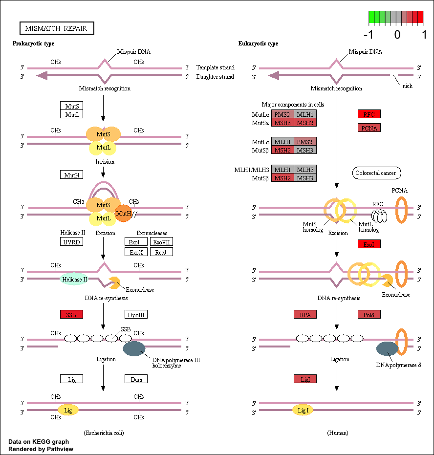
Now that we have our initial data loaded let’s choose a few pathways to visualize. The “Mismatch repair” repair pathway is significantly perturbed by up regulated genes, and corresponds to the following kegg id: “hsa03430”. We can view this using the row names of the pathway dataset fc.kegg.sigmet.p.up. Let’s use our experiment’s expression in the data frame tumor_v_normal_DE.fc and view it in the context of this pathway. Two graphs will be written to your current working directory by the pathview() function, one will be the original kegg pathway view and the second one will have expression values overlayed (see below). You can find your current working directory with the function getwd().

# View the hsa03430 pathway from the pathway analysis
fc.kegg.sigmet.p.up[grepl("hsa03430", rownames(fc.kegg.sigmet.p.up), fixed=TRUE),]

# Overlay the expression data onto this pathway
pathview(gene.data=tumor_v_normal_DE.fc, species="hsa", pathway.id="hsa03430")

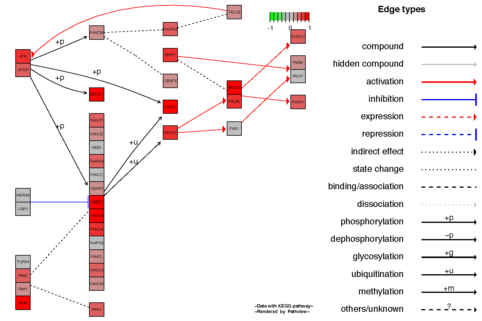
It is often nice to see the relationship between genes in the kegg pathview diagrams, this can be achieved by setting the parameter kegg.native=FALSE. Below we show an example for the Fanconi anemia pathway.

# View the hsa03430 pathway from the pathway analysis
fc.kegg.sigmet.p.up[grepl("hsa03460", rownames(fc.kegg.sigmet.p.up), fixed=TRUE),]

# Overlay the expression data onto this pathway
pathview(gene.data=tumor_v_normal_DE.fc, species="hsa", pathway.id="hsa03460", kegg.native=FALSE)
Pathway analysis | Griffith Lab

Genomic Visualization and Interpretations

Pathway analysis

In the previous section we examined differential expression of genes from the E-GEOD-50760 data set. In this section we will use the gage package to determine if there are any coordinated differential expression patterns in the data set we used for differential expression, E-GEOD-50760.

What is gage?

generally applicable gene-set enrichment (gage) is a popular bioconductor package for performing gene-set and pathway analysis. The package works independent of sample sizes, experimental designs, assay platforms, and is applicable to both microarray and rnaseq data sets. In this section we will use gage and gene sets from the “Kyoto Encyclopedia of Genes and Genomes” (KEGG) and “Gene Ontology” (GO) databases to perform pathway analysis. Let’s go ahead and install gage and load the differential expression results from the previous section.

# install gage
if (!requireNamespace("BiocManager", quietly = TRUE))
    install.packages("BiocManager")
BiocManager::install(c("gage","GO.db","AnnotationDbi","org.Hs.eg.db"), version = "3.8")
library(gage)

# load the differential expression results fro the previous section
load(url("http://genomedata.org/gen-viz-workshop/intro_to_deseq2/tutorial/deseq2Data_v1.RData"))

# extract the results from the deseq2 data
library(DESeq2)
tumor_v_normal_DE <- results(deseq2Data, contrast=c("tissueType", "primary colorectal cancer", "normal-looking surrounding colonic epithelium"))

setting up gene set databases

In order to perform our pathway analysis we need a list of pathways and their respective genes. The most common databases for this type of data are KEGG and GO. The gage package has two functions for querying this information in real time, kegg.gsets() and go.gsets(), both of which take a species as an argument and will return a list of gene sets and some helpful meta information for subsetting these list. For the KEGG database object kg.hsa$kg.sets stores all gene sets for the queried species; kg.hsa$sigmet.idx and kg.hsa$dise.idx store the indices for those gene sets which are classified as signaling and metabolism and disease respectively. We use this information to extract a list of gene sets for the signaling and metabolism and disease subsets. A similar process is used for the GO gene sets splitting the master gene set into the three gene ontologies: “Biological Process”, “Molecular Function”, and “Cellular Component”.

# set up kegg database
kg.hsa <- kegg.gsets(species="hsa")
kegg.sigmet.gs <- kg.hsa$kg.sets[kg.hsa$sigmet.idx]
kegg.dise.gs <- kg.hsa$kg.sets[kg.hsa$dise.idx]

# set up go database
go.hs <- go.gsets(species="human")
go.bp.gs <- go.hs$go.sets[go.hs$go.subs$BP]
go.mf.gs <- go.hs$go.sets[go.hs$go.subs$MF]
go.cc.gs <- go.hs$go.sets[go.hs$go.subs$CC]

annotating genes

We have our gene sets now however if you look at one of these objects containing the gene sets you’ll notice that each gene set contains a series of integers. These integers are actually entrez gene identifiers which presents a problem as our DESeq2 results use ensemble ID’s as gene identifiers. We will need to convert our gene identifiers to the same format before we perform the pathway analysis. Fortunately bioconductor maintains genome wide annotation data for many species, you can view these species with the OrgDb bioc view. This makes converting the gene identifiers relatively straight forward, below we use the mapIds() function to query the OrganismDb object for the gene symbol, entrez id, and gene name based on the ensembl id. Because there might not be a one to one relationship with these identifiers we also use multiVals="first" to specify that only the first identifier should be returned in such cases.

# load in libraries to annotate data
library(AnnotationDbi)
library(org.Hs.eg.db)

# annotate the deseq2 results with additional gene identifiers
tumor_v_normal_DE$symbol <- mapIds(org.Hs.eg.db, keys=row.names(tumor_v_normal_DE), column="SYMBOL", keytype="ENSEMBL", multiVals="first")
tumor_v_normal_DE$entrez <- mapIds(org.Hs.eg.db, keys=row.names(tumor_v_normal_DE), column="ENTREZID", keytype="ENSEMBL", multiVals="first")
tumor_v_normal_DE$name <- mapIds(org.Hs.eg.db, keys=row.names(tumor_v_normal_DE), column="GENENAME", keytype="ENSEMBL", multiVals="first")

Preparing DESeq2 results for gage

Before we perform the actuall pathway analysis we need to format our differential expression results into a format suitable for the gage package. Basically this means obtaining the normalized log2 expression values and assigning entrez gene identifiers to these values.

# grab the log fold changes for everything
tumor_v_normal_DE.fc <- tumor_v_normal_DE$log2FoldChange
names(tumor_v_normal_DE.fc) <- tumor_v_normal_DE$entrez

Running pathway analysis

We can now use the gage() function to obtain the significantly perturbed pathways from our differential expression experiment. By default the gage package performs this analysis while taking into account up and down regulation. Setting same.dir=FALSE will capture pathways perturbed without taking into account direction. This is generally not recommended for the GO groups as most genes within these gene sets are regulated in the same direction, however the same is not true for KEGG pathways and using this parameter may produce informative results in such cases.

Note on the abbreviations below: “bp” refers to biological process, “mf” refers to molecular function, and “cc” refers to cellular process. These are the three main categories of gene ontology terms/annotations.

# Run enrichment analysis on all log fc
fc.kegg.sigmet.p <- gage(tumor_v_normal_DE.fc, gsets = kegg.sigmet.gs)
fc.kegg.dise.p <- gage(tumor_v_normal_DE.fc, gsets = kegg.dise.gs)
fc.go.bp.p <- gage(tumor_v_normal_DE.fc, gsets = go.bp.gs)
fc.go.mf.p <- gage(tumor_v_normal_DE.fc, gsets = go.mf.gs)
fc.go.cc.p <- gage(tumor_v_normal_DE.fc, gsets = go.cc.gs)

# covert the kegg results to data frames
fc.kegg.sigmet.p.up <- as.data.frame(fc.kegg.sigmet.p$greater)
fc.kegg.dise.p.up <- as.data.frame(fc.kegg.dise.p$greater)

fc.kegg.sigmet.p.down <- as.data.frame(fc.kegg.sigmet.p$less)
fc.kegg.dise.p.down <- as.data.frame(fc.kegg.dise.p$less)

# convert the go results to data frames
fc.go.bp.p.up <- as.data.frame(fc.go.bp.p$greater)
fc.go.mf.p.up <- as.data.frame(fc.go.mf.p$greater)
fc.go.cc.p.up <- as.data.frame(fc.go.cc.p$greater)

fc.go.bp.p.down <- as.data.frame(fc.go.bp.p$less)
fc.go.mf.p.down <- as.data.frame(fc.go.mf.p$less)
fc.go.cc.p.down <- as.data.frame(fc.go.cc.p$less)

Which genes are in > 30% of significant pathways in the upregulated GO biological process results (q <= .05)

Two genes are, ATM, CCNB1. Here is an Rscript to get the correct answer.