arranging plots with ggplot2*
We’ve gone over the basics of ggplot2 in the previous section, in this section we will go over some tecniques to create multi-panel figures within R.
Creating initial plots
Often when creating figures for publications the figure in the final manuscript is actually composed of multiple figures. You could of course achieve this using third-party programs such as illustrator and inkscape however that means having to manually redo the figure in those programs anytime there is an update or change. Instead of going through that hassel let’s learn how to do it all programatically. To achieve this we will of course make our plots using ggplot, the gtable package to manipulate the plots post-creation, and the gridExtra package to do the actual aligning. Let’s go ahead and get started.
Our first step is to make some plots. We’ll go ahead and use the same dataset as before which is available at http://genomedata.org/gen-viz-workshop/intro_to_ggplot2/ggplot2ExampleData.tsv as a reminder. Let’s go ahead and load this data in, if it isn’t in R already.
# install the ggplot2 library and load it
library(ggplot2)

# load Data
variantData <- read.delim("http://genomedata.org/gen-viz-workshop/intro_to_ggplot2/ggplot2ExampleData.tsv")
Next we’ll make a bar chart for the genes which have over 20 mutations in all samples. The commands here should be review from previous sections. If you’re having problems following refer back to the introduction to R and ggplot2 sections.
# install the plyr library
library(plyr)

# count the number of variants for each gene/mutation type and format for ggplot
geneCount <- count(variantData, vars=c("gene_name", "type"))
head(geneCount, 10)
geneCount <- geneCount[geneCount$freq > 20,]

# to order samples for ggplot also get a total count overall (SNPs + InDels)
geneCountOverall <- aggregate(data=geneCount, freq ~ gene_name, sum)
geneOrder <- geneCountOverall[order(geneCountOverall$freq),]$gene_name
geneCount$gene_name <- factor(geneCount$gene_name, levels=geneOrder)

# make the barchart
p1 <- ggplot() + geom_bar(data=geneCount, aes(x=gene_name, y=freq, fill=type), stat="identity") + xlab("Gene") + ylab("Frequency") + scale_fill_manual("Mutation", values=c("#F97F51", "#55E6C1")) + theme_bw() + theme(plot.background = element_rect(color="red", size=2))
p1
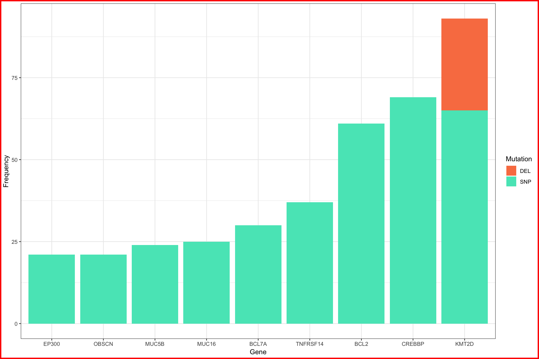
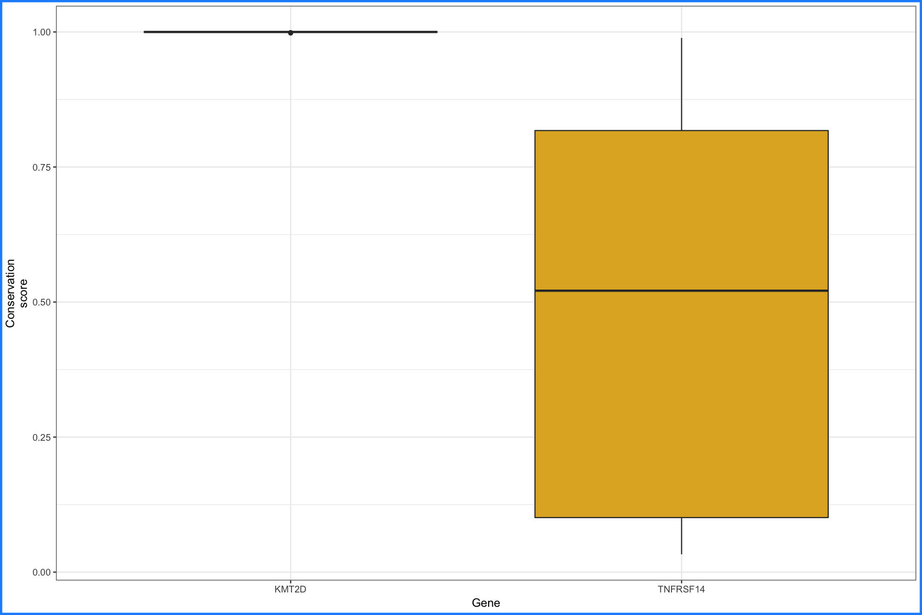
We can see from the p1 plot that KMT2D seems interesting, it’s got the most mutations and a fair number of deletions as well. To explore this a bit further lets go ahead and compare KMT2D to a few of the other highly mutated genes from our first plot. To do this we’ll make a boxplot for the genes KMT2D and TNFRSF14 comparing the conservation score. This metric comes from UCSC in our data and is essentially a score from 0-1 of how conserved a region is across vertebrates. A high score would mean the region is highly conserved and probably an important region of the genome.
geneCompare1 <- variantData[variantData$gene_name %in% c("KMT2D", "TNFRSF14"),]
geneCompare1 <- geneCompare1[,c("gene_name", "trv_type", "ucsc_cons")]
geneCompare1 <- geneCompare1[geneCompare1$trv_type == "missense",]
geneCompare1$ucsc_cons <- as.numeric(as.character(geneCompare1$ucsc_cons))
p2 <- ggplot() + geom_boxplot(data=geneCompare1, aes(x=gene_name, y=ucsc_cons, fill=gene_name)) + scale_fill_manual("Gene", values=c("#e84118", "#e1b12c")) + theme_bw() + xlab("Gene") + ylab("Conservation\nscore") + theme(plot.background = element_rect(color="dodgerblue", size=2))
p2
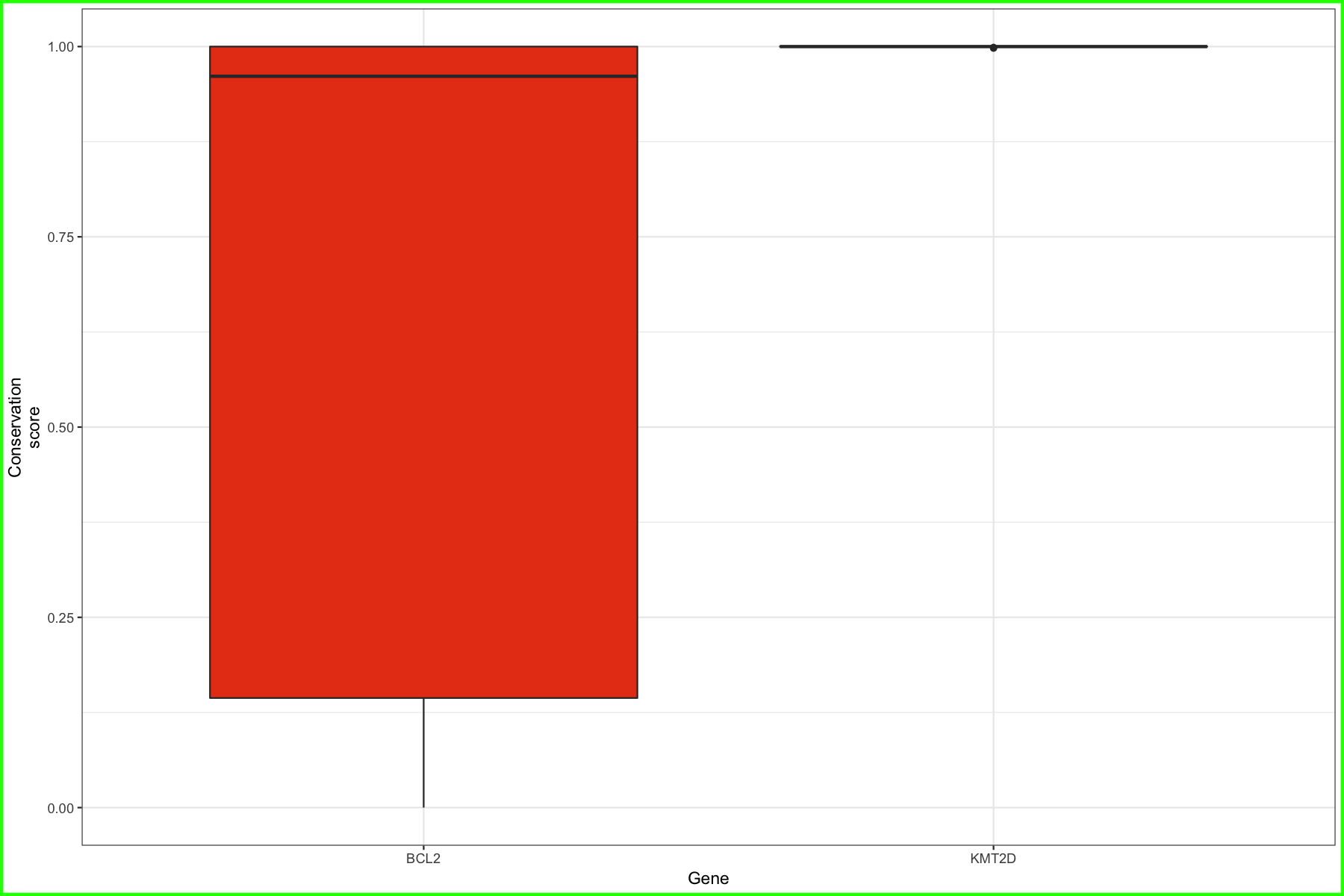
And we’ll go ahead and do the same thing for KMT2D and BCL2.
geneCompare2 <- variantData[variantData$gene_name %in% c("KMT2D", "BCL2"),]
geneCompare2 <- geneCompare2[,c("gene_name", "trv_type", "ucsc_cons")]
geneCompare2 <- geneCompare2[geneCompare2$trv_type == "missense",]
geneCompare2$ucsc_cons <- as.numeric(as.character(geneCompare2$ucsc_cons))
p3 <- ggplot() + geom_boxplot(data=geneCompare2, aes(x=gene_name, y=ucsc_cons, fill=gene_name)) + scale_fill_manual("Gene", values=c("#e84118", "#4cd137")) + theme_bw() + xlab("Gene") + ylab("Conservation\nscore") + theme(plot.background = element_rect(color="green", size=2))
p3
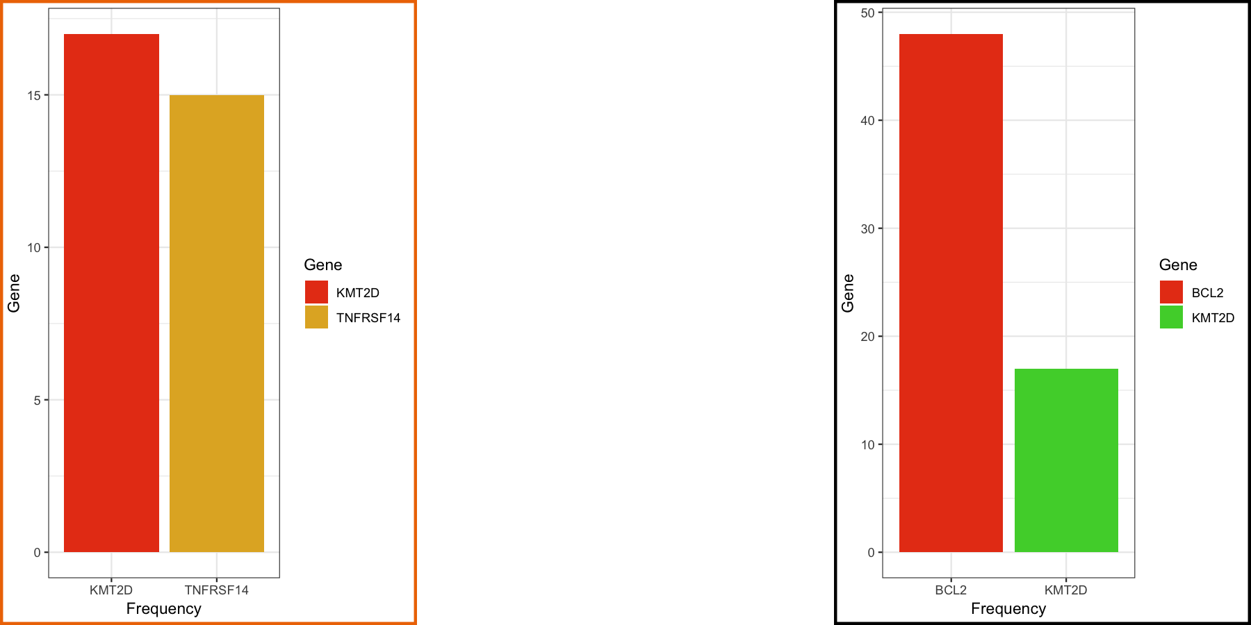
We have our boxplots for missense mutations, it would be nice to know how many data points make up those boxplots as well. To do this we will just create two quick barcharts counting the mutations in the plots defined above.
p4 <- ggplot() + geom_bar(data=geneCompare1, aes(x=gene_name, fill=gene_name)) + scale_fill_manual("Gene", values=c("#e84118", "#e1b12c")) + theme_bw() + theme(plot.background = element_rect(color="darkorange2", size=2)) + xlab("Gene") + ylab("Frequency")
p4

p5 <- ggplot() + geom_bar(data=geneCompare2, aes(x=gene_name, fill=gene_name)) + scale_fill_manual("Gene", values=c("#e84118", "#4cd137")) + theme_bw() + theme(plot.background = element_rect(color="black", size=2)) + xlab("Gene") + ylab("Frequency")
p5
Arranging plots
With our initial plots created wouldn’t it be nice if we could plot these all at once. The good news is that we can. There are a number of packages for available to achieve this. Currently the most widley used are probably gridExtra, cowplot, and egg. In this course we will use gridExtra; before working on our own data, let’s illustrate some basic concepts in gridExtra. Below we will load the grid library in order to create some visual objects to visualize, and use the gridExtra library to arrange these plots. We then create our objects to visualize, grob1-grob4. Theres no need to understand how these objects are created, this is just done to have something intuitive to use when arranging. Our next step is to create the layout for arrangment, we do this by creating a matrix where each unique element in the matrix (1, 2, 3, 4) corresponds to one of our objects to visualize. For example in the layout we use below we have 3 rows and 4 columns in which to place our visualizations. We specify the first row should all be one plot, the second row should be split between plots 2 and 3, and the third row should be split between plots 2 and 4. We then pass grid.arrange our objects to plot and the layout, so in this case grob1 corresponds to the element 1 in the matrix since grob1 is supplied first to grid.arrange.
# make objects to illustrate gridExtra functionality
library(grid)
library(gridExtra)

# make objects to visualize
# you can view these by doing grid.draw(grob1)
grob1 <- grobTree(rectGrob(gp=gpar(fill="#EE5A24", alpha=1)), textGrob("1", gp=gpar(fontsize=28)))
grob2 <- grobTree(rectGrob(gp=gpar(fill="#009432", alpha=1)), textGrob("2", gp=gpar(fontsize=28)))
grob3 <- grobTree(rectGrob(gp=gpar(fill="#0652DD", alpha=1)), textGrob("3", gp=gpar(fontsize=28)))
grob4 <- grobTree(rectGrob(gp=gpar(fill="#833471", alpha=1)), textGrob("4", gp=gpar(fontsize=28)))

# create layout for arrangement and do the arrangement
layout <- rbind(c(1, 1, 1, 1),
                c(2, 2, 3, 3),
                c(2, 2, 4, 4))
grid.arrange(grob1, grob2, grob3, grob4, layout_matrix=layout)
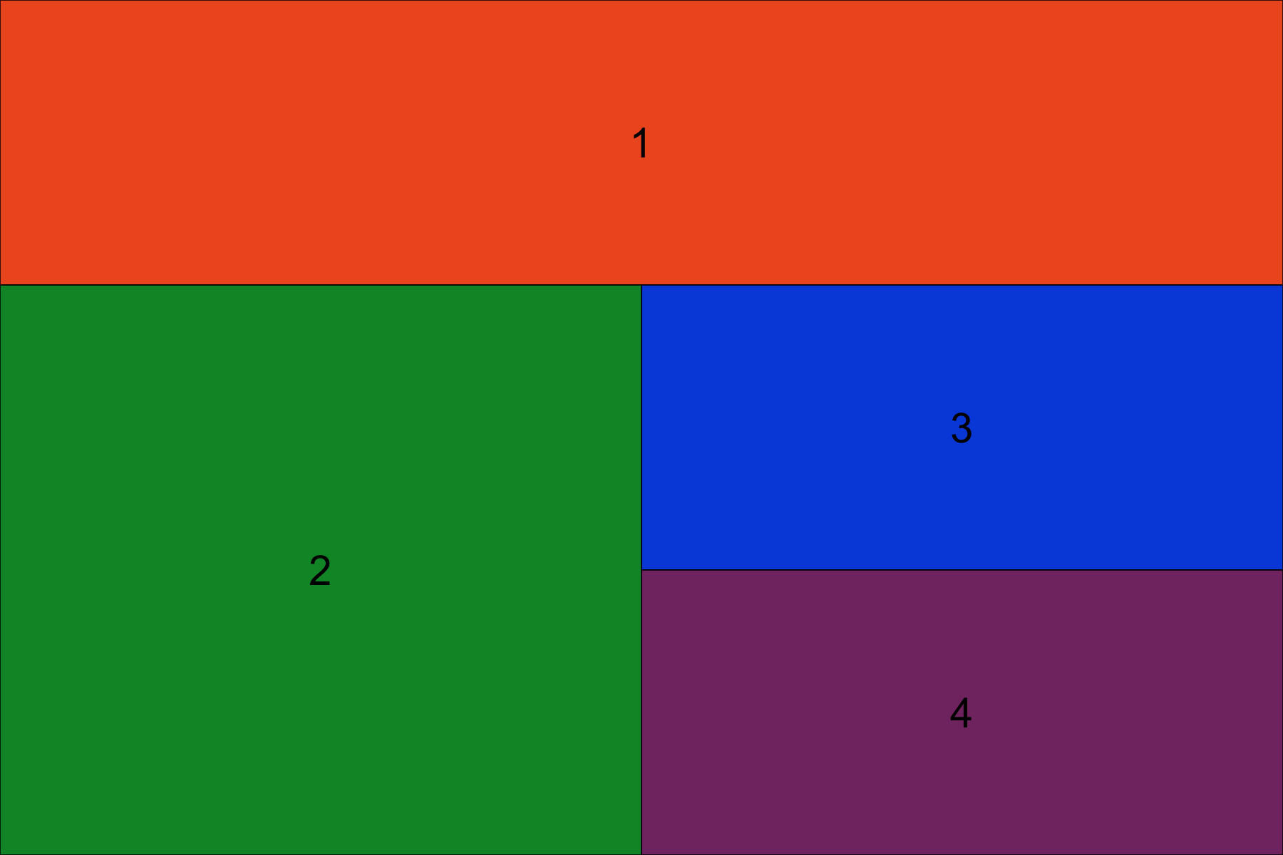
Note how the numbers above in the rbind expression correspond to the layout produced. The first row has object 1 spanning across four columns. The second row is split eveny between object 2 and 3. The third row is split evenly between object 2 and 4.
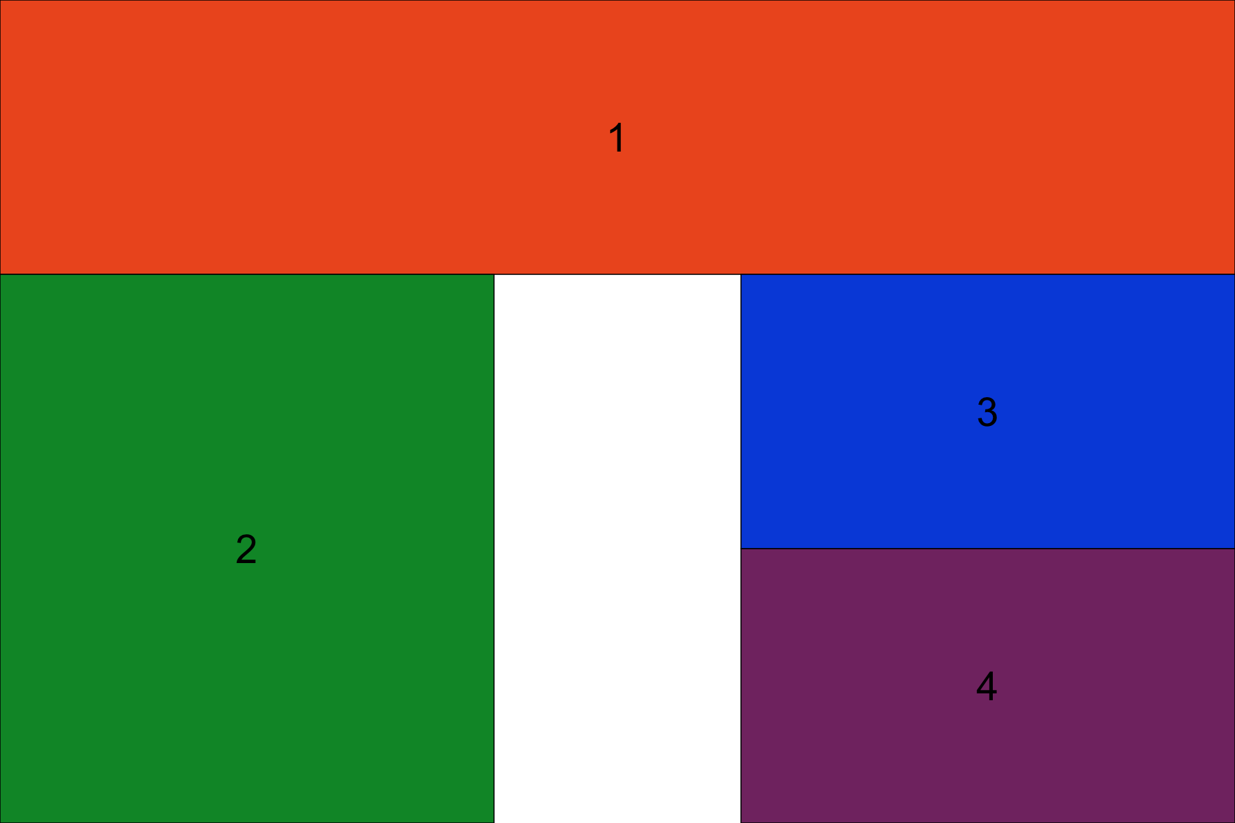
It is also possible to add empty cells in our layout by inserting NA into our layout matrix. Below we split out grob2 from grob3 and grob4.
layout <- rbind(c(1, 1, 1, 1, 1),
                c(2, 2, NA, 3, 3),
                c(2, 2, NA, 4, 4))

grid.arrange(grob1, grob2, grob3, grob4, layout_matrix=layout)
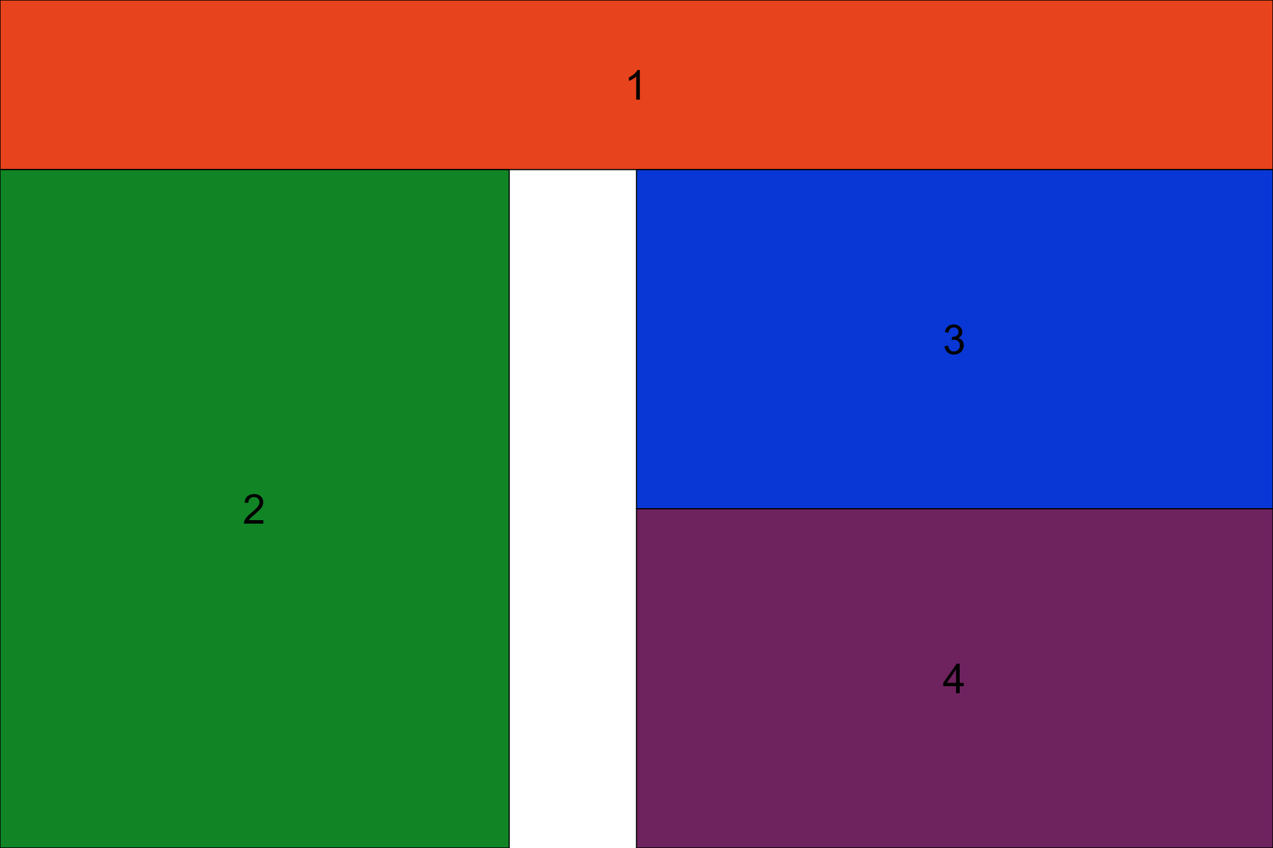
We can also adjust the size of element relative to our layout matrix. For example, below we say that each row (there are 3), should take up 20%, 40% and 40% of the arranged plot respectively.
layout <- rbind(c(1, 1, NA, 1, 1),
                c(2, 2, NA, 3, 3),
                c(2, 2, NA, 4, 4))

grid.arrange(grob1, grob2, grob3, grob4, layout_matrix=layout, widths=c(.2, .2, .1, .3, .2), heights=c(.2, .4, .4))
There is much more information on how gridExtra works in the various gridExtra vignettes, obviously it is a powerful package for arranging plots. Let’s try an exercise to reinforce the concepts we’ve just learned. Try recreating the plot below:
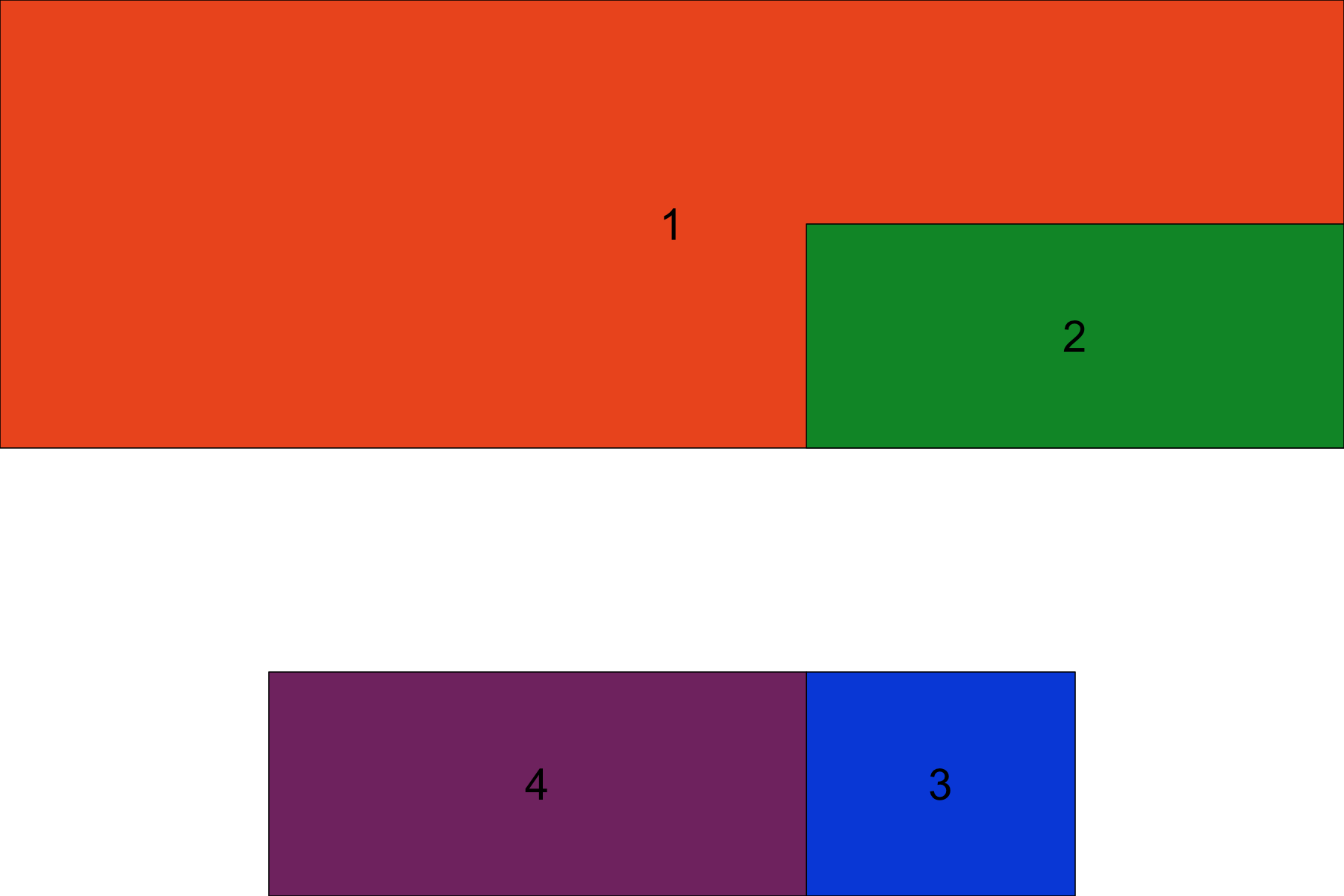
Get a hint!
the layout matrix should be 5 columns by 4 rows
solution
The solution is in solution.R
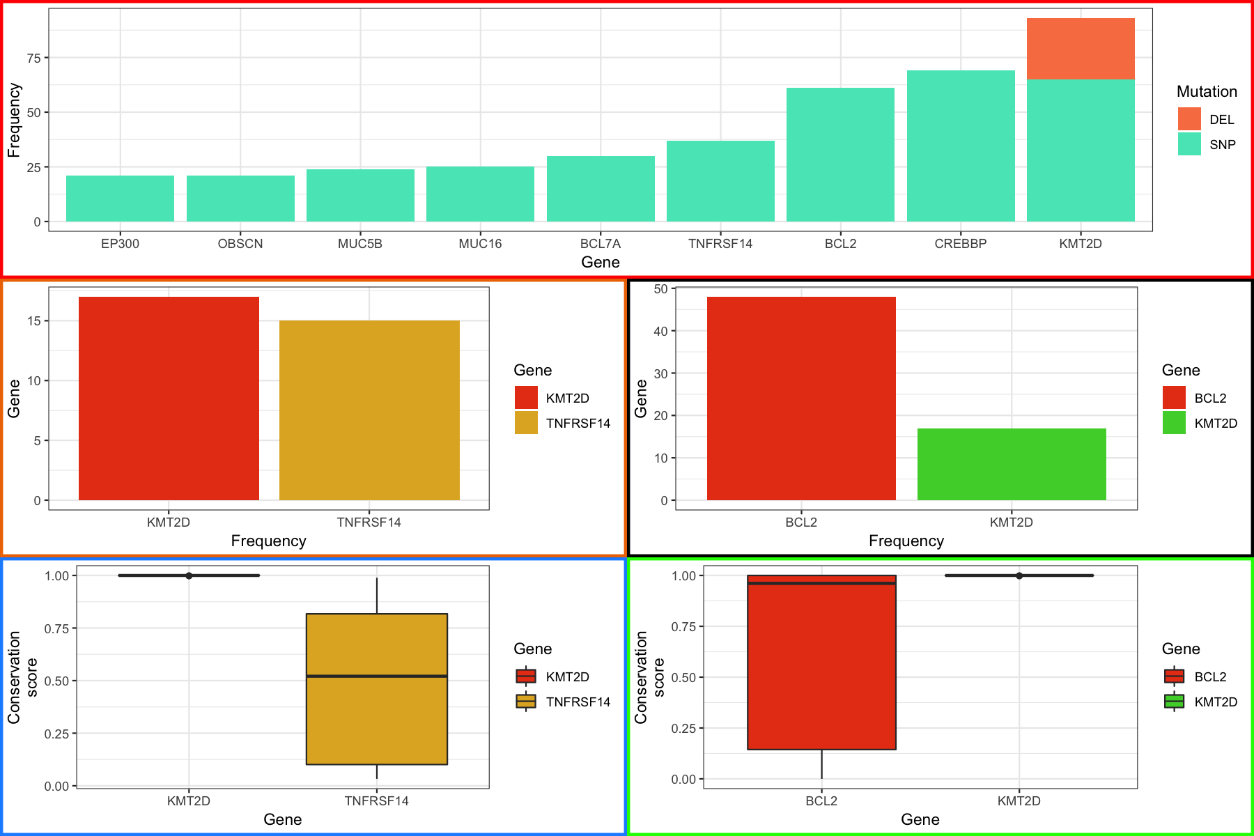
Now that we understand the basics of how gridExtra works let’s go ahead and make an attempt at a multi-panel figure. We’ll put the main barchart on top, and match the boxplots with their specific barcharts on rows 2 and 3 of a layout. At the end you should see something like the figure below. Note that for this exercise each plot has a colored border to help visualize the layout. To make the plot cleaner we would drop that by removing the “theme(plot.background = element_rect()” entries above when each plot is generated.
layout <- rbind(c(1, 1),
                c(2, 3),
                c(4, 5))
grid.arrange(p1, p4, p5, p2, p3, layout_matrix=layout)
More advanced topics related to this section are included in the course appendix here.