Introduction to copy number spectrum plots
A common task in any bioinformatic analysis of next generation sequencing data is the the determination of copy number gains and losses. The cnSpec() function, short for “copy number spectrum”, from the GenVisR package is designed to provide a view of copy number calls for a cohort of cases. It is very similar to the cnFreq() function discussed in the previous section but displays per sample copy number changes in the form of a heatmap instead of summarizing calls. In this section we will use cnSpec() to explore the copy number calls from the same data set of her2 positive breast cancer samples used in the previous section.
Loading data
The data we will be working with was generated with the R package Copycat2. The output of this program consists of a file containing segmented copy number calls. You can find these files on http://genomedata.org/gen-viz-workshop/GenVisR/, go ahead and download all files with a “.cc2.tsv” extension. Once these files are downloaded we will need to read them into R and coerce them into a single data frame with column names “chromosome”, “start”, “end”, “segmean”, and “sample”. As a first step install and load the stringr package we’ll need this to make some of the string manipulation we’ll be doing easier. Once stringr is loaded run through the rest of the R code below the details of which can be found in the previous section.
# load extra libraries
# install.packages("stringr")
library("stringr")

# get locations of all cn files
files <- Sys.glob("~/Desktop/*cc2.tsv")

# create function to read in and format data
a <- function(x){
    # read data and set column names
    data <- read.delim(x, header=FALSE)
    colnames(data) <- c("chromosome", "start", "end", "probes", "segmean")

    # get the sample name from the file path
    sampleName <- str_extract(x, "H_OM.+cc2")
    sampleName <- gsub(".cc2", "", sampleName)
    data$sample <- sampleName

    # return the data
    return(data)
}

# run the anonymous function defined above
cnData <- lapply(files, a)

# turn the list of data frames into a single data frame
cnData <- do.call("rbind", cnData)
Creating an initial plot
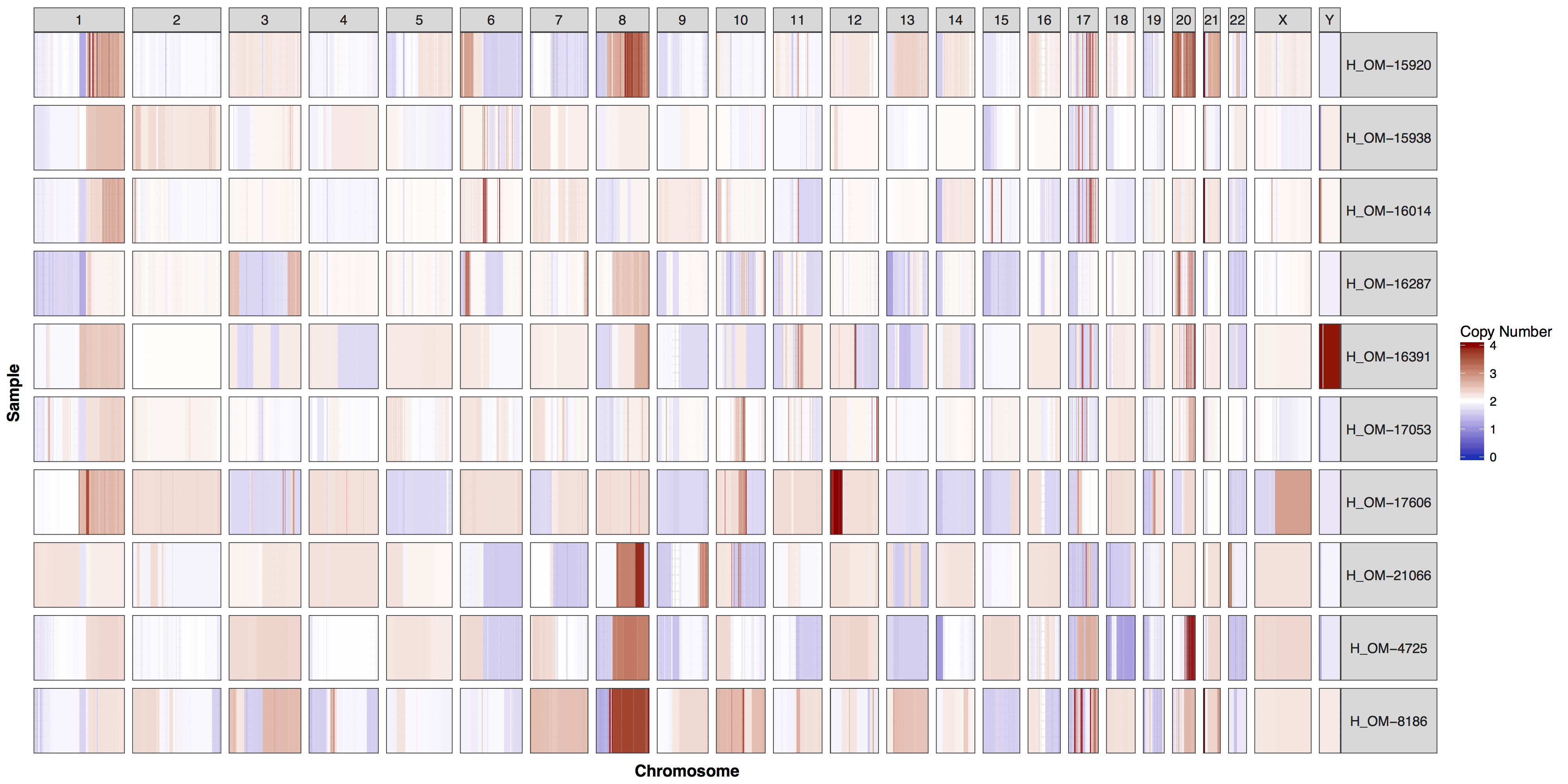
Similar to cnFreq() in cnSpec() the only required parameters are a data frame with column names “chromosome”, “start”, “end”, “segmean”, “sample” and passing a reference assembly to the parameter genome=, one of “hg19”, “hg38”, “mm9”, “mm10”, or “rn5”. However cnSpec() is also more flexible and can accept custom coordinates with the parameter y, allowing it to plot any completed reference assembly. Fortunately for us when you installed the GenVisR package you also installed a data set called cytoGeno which contains the coordinates of cytogenetic bands for 5 reference assemblies. Let’s use this data set to pass in our genomic boundaries for “hg19” into the parameter y and construct an initial plot.
# construct genomic boundaries from cytoGeno
genomeBoundaries <- aggregate(chromEnd ~ chrom, data=cytoGeno[cytoGeno$genome=="hg19",], max)
genomeBoundaries$chromStart <- 0
colnames(genomeBoundaries) <- c("chromosome", "end", "start")

# create the plot
cnSpec(cnData, y=genomeBoundaries)
The genome parameter
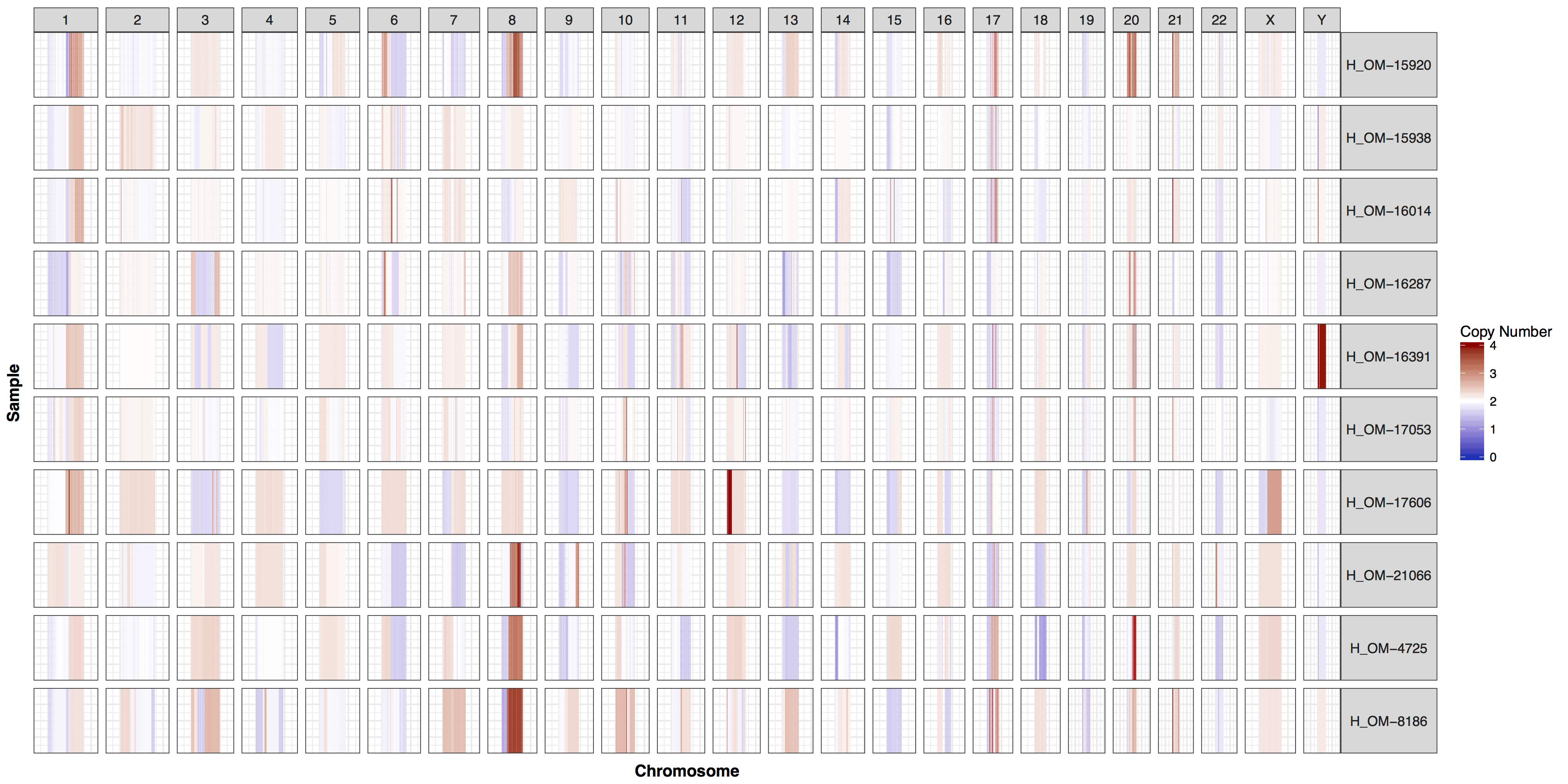
These plots are fairly straightforward, but it is helpful to know what the genome and y parameters actually do. As eluded to in the previous section only one of these is required, as they both do the same thing, define genome boundaries. This is done to ensure that if you only had data for one section of a chromosome the entire chromosome space is still plotted. To get a sense of what is actually happening let’s add a flank to genomeBoundaries and see what happens. You’ll see in the plot below that all the chromosomes plotted below now have a padding where no data is plotted.
# add a flank to the genomic coordinates
genomeBoundaries_2 <- genomeBoundaries
genomeBoundaries_2$start <- genomeBoundaries_2$start - 1e8
genomeBoundaries_2$end <- genomeBoundaries_2$end + 1e8

# create a plot
cnSpec(cnData, y=genomeBoundaries_2)
Exercises
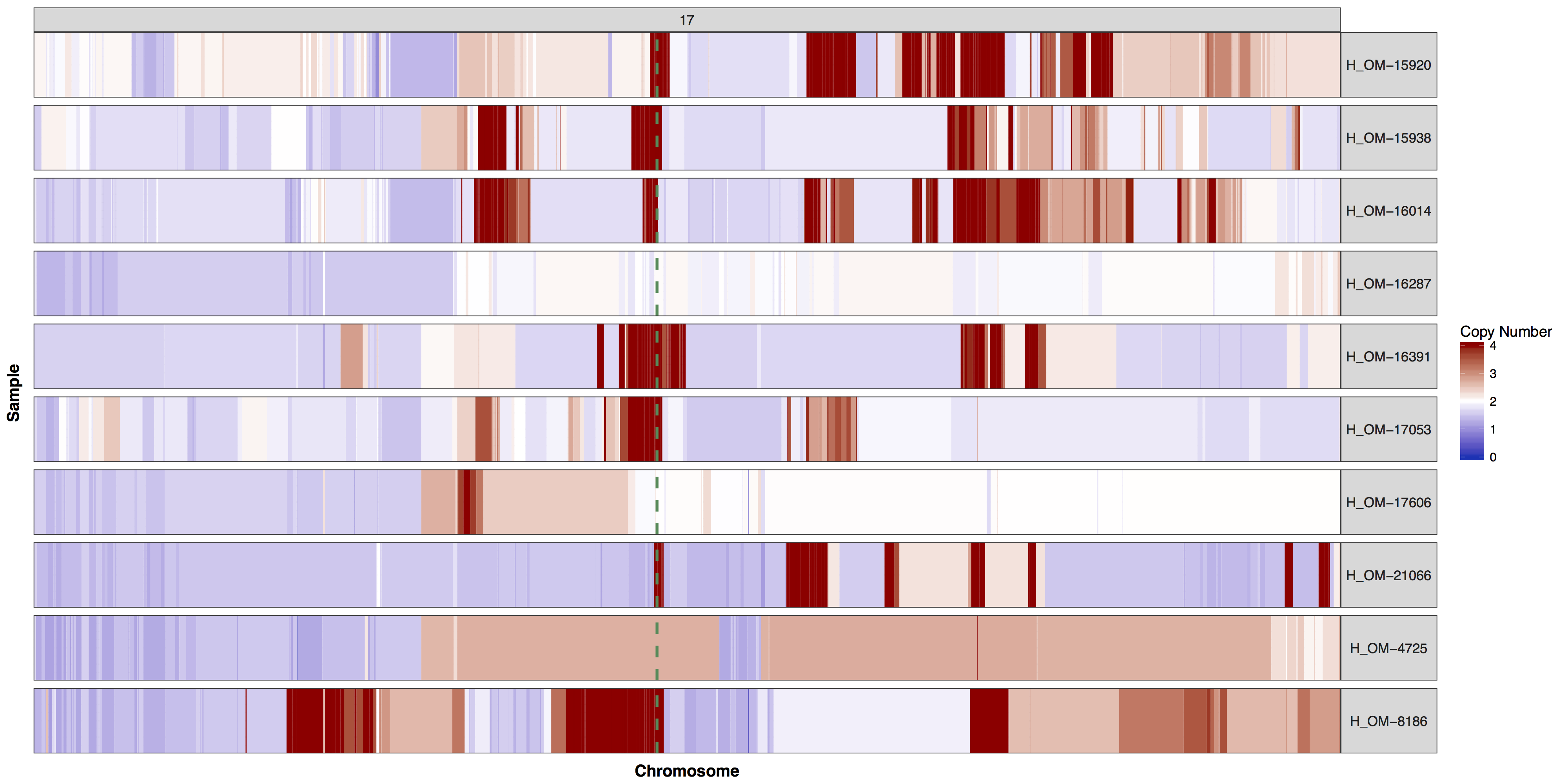
There are times when a genome wide view of copy number changes is not necessary or desireable, for example we may want to view just chromosome 17 to look for ERBB2 amplifications as these are HER2+ breast cancer samples. We can achieve this by creating a custom genome to input into the y parameter. Try using what you know to only plot chromosome 17 and use geom_vline() to highlight were ERBB2 is located. You can pass additional plot layers to cnSpec() with the param plotLayer. Your plot should look something like the one below.
Get a hint!
You'll need to create a custom genome that is only chromosome 17, you'll need to subset your input data as well.
Answer
cnSpec(cnData[cnData$chromosome=="17",], y=genomeBoundaries[genomeBoundaries$chromosome=="chr17",], plotLayer=geom_vline(xintercept = 39709170, colour="seagreen4", size=1, linetype=2))
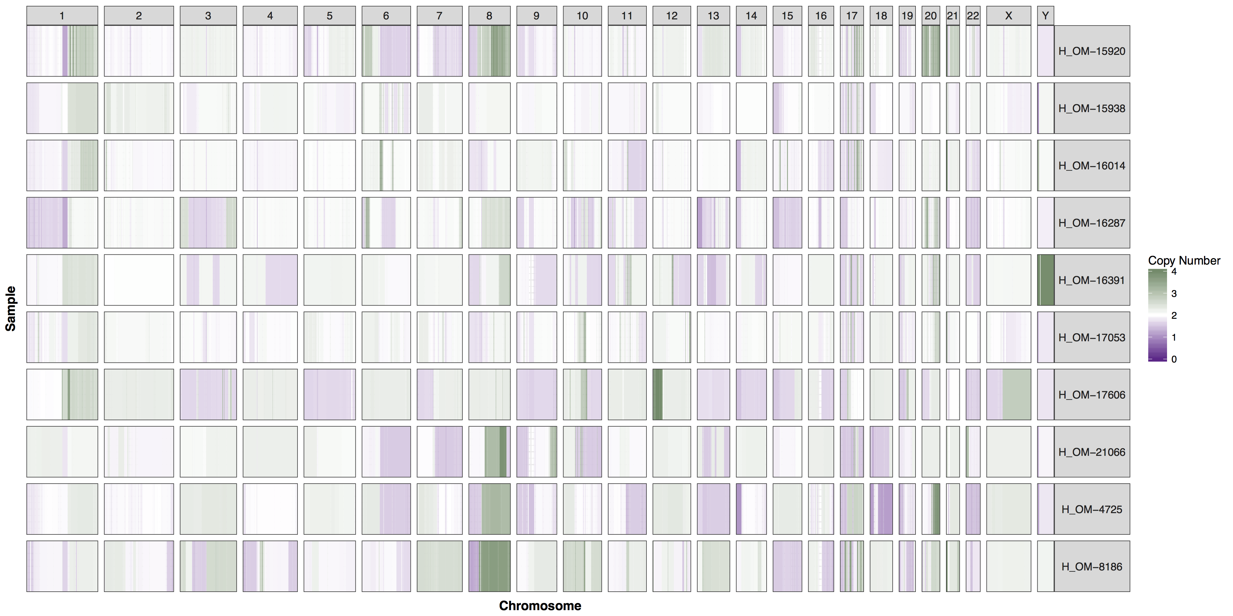
You could of course add whichever layers you wish to change any aspect of the plot’s we’ve been producing, however you will often find parameters within GenVisR functions in order to make the most common changes. Try reading the documentation for cnSpec() and create a version of the plot below.
Get a hint!
One of the parameters is "CN_Loss_colour"
Answer
cnSpec(cnData, y=genomeBoundaries, CN_Loss_colour="darkorchid4", CN_Gain_colour = "darkseagreen4")