Introduction to R

Over this tutorial series, we will be using R extensively, the language underlying graphical programs ggplot2, ggvis, and GenVisR. We highly recommend familiarity with R for all students. This page is intended to provide a brief overview of R. However, there are a myriad of resources available that we recommend to supplement the information given here (See Additional Resources below).

R and Rstudio

R is an open source functional programming language developed for statistical computing and graphics. The language includes a number of features that make it ideal for data analysis and visualization and is the primary computing language used in this course.

RStudio in an open source integrated development environment (IDE) written and maintained by RStudio for the R programming language. It is available on all major operating systems and contains a number of features designed to make writing and developing R code more efficient. These features include debugging tools, auto-complete, and syntax highlighting.

Installation

R

To use R go to https://www.r-project.org/, select a mirror via the CRAN link located on the top right, download the appropriate binary distribution for your operating system, and follow the on screen instructions when opening the downloaded file. Once R is installed you can call the function sessionInfo() to view the version of R and all loaded packages.

Rstudio

Rstudio can be downloaded at https://www.rstudio.com/, select the Products->Rstudio tab within the navigation links at the top, then download the “RStudio Desktop - Open Source Edition”, and follow the on screen instructions. Rstudio will automatically detect the current R on your operating system and call the R executable on startup.

CRAN and Bioconductor

CRAN

Part of what makes R an attractive option for data analysis and visualization is the support it receives from a large community of developers. Part of this support comes from users adding new functionality to core R via functions and data through packages. The Comprehensive R Archive network (CRAN) is a network of servers that stores R, documentation, and many of the packages available for R. To date there are 14,037 packages on CRAN, these packages can be installed by running the install.packages() command in an R terminal. For example, to install the ‘plyr’ package, run the following command in an R terminal:

# Install the plyr package by Hadley Wickham
install.packages("plyr")

An R package is a collection of functions, data and compiled code. Once a package is installed, it still needs to be loaded into memory before use. The library() function is used to load a package into memory. Once loaded, the functions and datasets of the package can be used.

sessionInfo()
library(plyr)
sessionInfo()

What do you see by executing sessionInfo() twice?

To see what packages are currently available in your R installation you can do the following:

# Where package files are installed on your computer
.libPaths()

# All packages currently installed
lapply(.libPaths(), dir)

Bioconductor

Bioconductor is another archive of R packages specific to bioinformatics and genomics. This archive is maintained by the Bioconductor core team and is updated bi-annually. To date, there are 2,974 packages available via bioconductor. Packages are categorized within biocViews as ‘Software’, ‘AnnotationData’, and ‘ExperimentData.’ You can explore the packages available on this webpage by searching within these tags, categorizing packages based upon relevant topics or types of analysis. Bioconductor packages are managed and installed using the BiocManager() function. Note that the BiocManager function must be installed before trying to install any Bioconductor packages. Bioconductor packages can be installed by running the following in an R terminal:

# Install biocmanager if it's not already there
if (!requireNamespace("BiocManager"))
    install.packages("BiocManager")

# Install core bioconductor packages
BiocManager::install()

# Install specific bioconductor packages
BiocManager::install("GenomicFeatures")

# Upgrade installed bioconductor packages
BiocManager::install()

Common file type extensions in R/Rstudio

• .R This is the primary file extension in R and denotes a file containing R code.
• .Rproj Denotes an R project file, these are commonly used when developing R libraries in Rstudio but are useful for analysis projects as well. Essentially they store saved settings in Rstudio.
• .Rdata These files are R data files and are used to store data in a compressed format that are easily exported from and loaded in to R. They store R objects and are useful if for example your R script takes awhile to run and you want to store results to avoid having to rerun the script.
• .Rmd Denotes Rmarkdown files, Rmarkdown provides a way to include R code and results within a markdown document. Commonly used to present results in a convenient format and/or to document code in a more user readable way.
• .Rnw Denotes a sweave file, similar to markdown it provides a way to intersperse texts, plots, and code in one document. The main difference being that instead of markdown syntax, LaTeX is used instead.

Documentation and example data in R

As with any software, documentation is key to the usefulness for a user. R makes finding documentation very easy. In order to find the documentation for a specific function where you have already loaded the library, simple enter “?” followed by the function name. This will pull up a manual specific to that function. If you have the library for a function installed but not loaded entering “??” will also pull up the relevant documentation. In either case, the function’s documentation immediately appears in the ‘Help’ tab of the lower right window of the screen. In addition, many packages have additional documentation in the form of vignettes. To view these vignettes from R use the vignette() function, specifying the package name within the function call (e.g. vignette(“grid”)). The source code for any function in R can also be viewed by typing the function name into R without any parameters or parentheses.

R also has a variety of datasets pre-loaded. In order to view these, type data() in your R terminal. We will be using a few of these data sets to illustrate key concepts in this lesson.

Assignment and data types

When working in any programming language, values are stored as variables. Defining a variable tells the language to allocate space in memory to store that variable. In R, a variable is assigned with the assignment operator “<-“ or “=”, which assigns a value to the variable in the user workspace or the current scope respectively. For the purposes of this course, assignment should always occur with the “<-“ operator. All variables are stored in objects. The least complex object is the atomic vector. Atomic vectors contain values of only one specific data type. Atomic vectors come in several different flavors (object types) defined by their data type. The six main data types (and corresponding object types) for atomic vectors are: “double (numeric)”, “integer”, “character”, “logical”, “raw”, and “complex”. The data type can be checked with the typeof() function. The object type can be checked with the class() function. Alternatively, data type and object type can also be checked with the is.() family of functions which will return a logical vector (True/False). Object and data types can also be coerced from one type to another using the as.() family of functions. An example of each data type is shown below. In each case we will check the object and data type. We will also try coercing some objects/data from one type to another. Understanding and moving between data/object types is important because many R functions expect inputs to be of a certain type and will produce errors or unexpected results if provided with the wrong type.

# numeric
foo <- 1.0
foo
is.numeric(foo)
is.double(foo)
typeof(foo)
class(foo)

# integer values are defined by the "L"
bar <- 1L
bar
is.integer(bar)
typeof(bar)
class(bar)

# character, used to represent text strings
baz <- "a"
baz
is.character(baz)
typeof(baz)
class(baz)

# logical values are either TRUE or FALSE
qux <- TRUE
qux
is.logical(qux)
typeof(qux)
class(qux)

# the charToRaw() function is used to store the string in a bit format
corge <- charToRaw("Hello World")
corge
is.raw(corge)
typeof(corge)
class(corge)

# complex
grault <- 4 + 4i
grault
is.complex(grault)
typeof(grault)
class(grault)

#Try coercing foo from a numeric vector with data type double to an integer vector
fooi <- as.integer(foo)
fooi
typeof(fooi)
class(fooi)

Data structures (objects)

Data structures in R are objects made up of the data types mentioned above. The type of data structure is dependent upon the homogeneity of the stored data types and the number of dimensions. Commonly used data structures include vectors, lists, matrices, arrays, factors, and dataframes. The most common data structure in R is the vector, which contains data in 1 dimension. There are two types: atomic vectors (discussed above), which contain one data type (i.e. all numeric, all character, etc.) and lists, which contain multiple data types. Atomic vectors are created with the c() function. Recall from above that the data type contained within an atomic vector can be determined using the typeof() function and the type of data object/structure determined with class() function. These functions can also be used on more complex data structures. Vectors in R can be sliced (extracting a subset) with brackets [], using either a boolean vector or a numeric index. Conditional statements together with the which function can also be use to quickly extract subsets of a vector that meets certain conditions.

# Create an atomic vector
vec <- c(2,3,5:10,15,20,25,30)

# Test that it is atomic, of object type numeric, and report the data and object type
is.atomic(vec)
is.numeric(vec)
typeof(vec)
class(vec)

# Coerce the numeric vector to character
vec <- as.character(vec)
is.character(vec)

# Extract the first element of the vector
vec[1]

# Determine which element of the vector contains a "5"
vec == "5"

# Extract the character 5
vec[vec == "5"]

# Determine which index of the vector contains a "5"
which(vec == "5")

# Extract the elements of the vector with that index
vec[which(vec == "5")]

# Coerce back to numeric
vec <- as.numeric(vec)

# Determine which elements of the vector are >= 5
vec >= 5

# Combine conditional expressions
# Determine which elements of the vector are <=5 OR >=20
vec <= 5 | vec >= 20

# Determine which elements of the vector are >=5 AND <=20
vec >= 5 & vec <= 20

# Determine the indices of the vector with values >=5 AND <=20, then extract those elements
which(vec >= 5 & vec <= 20)
vec[which(vec >= 5 & vec <= 20)]

# Do something similar, using which() but for a matrix.
# Create a 5x10 matrix where values are randomly 1:10
x <- sample(1:10, size = 50, replace=TRUE)
a <- matrix(x, nrow=5)

# Find all the elements of that matrix that are '3'
which(a==3, arr.ind=TRUE)

Lists are created using the list() function and are used to make more complicated data structures. As mentioned, lists can be heterogeneous, containing multiple data types, objects, or structures (even other lists). Like vectors, items from a list can also be extracted using brackets []. However, single brackets [] are used to return an element of the list as a list. Double brackets [[]] are used to return the the designated element from the list. In general, you should always use double brackets [[]] when you wish to extract a single item from a list in its expected type. You would use the single brackets [] if you want to extract a subset of the list.

# create list and verify its data and object type
myList <- list(c(1:10), matrix(1:10, nrow=2), c("foo", "bar"))
typeof(myList)
class(myList)

# extract the first element of the list (the vector of integers)
myList[[1]]
typeof(myList[[1]])
class(myList[[1]])

# extract a subset (e.g., the first and third items) of the list into a new list
myList[c(1,3)]

It is important to address attributes in our discussion of data structures. All objects can contain attributes, which hold metadata regarding the object. An example of an attribute for vectors are names. We can give names to each element within a vector with the names() function, labeling each element of the vector with a corresponding name in addition to its index. Another type of data structure is a factor, which we will use extensively in ggplot2 to define the order of categorical variables. Factors hold metadata (attributes) regarding the order and the expected values. A factor can be specifically defined with the function factor(). The expected values and order attributes of a factor are specified with the “levels” param.

# create a named vector
vec <- c("foo"=1, "bar"=2)

# change the names of the vector
names(vec) <- c("first", "second")

# coerce the vector to a factor object
vec <- factor(vec, levels=c(2, 1))

Importing and exporting data

As we have seen, data can be created on the fly in R with the various data structure functions. However it is much more likely that you will need to import data into R to perform analysis. Given the number of packages available, if a common filetype exists (XML, JSON, XLSX), R can probably import it. The most common situation is a simple delimited text file. For this the read.table() function and its various deriviatives are immensely useful. Type in ?read.table in your terminal for more information about its usage. Once data has been imported and analysis completed, you may need to export data back out of R. Similar to read.table(), R has functions for this purpose. write.table() will export the data given, in a variety of simple delimited text files, to the file path specified. See ?write.table for more information. Two common issues with importing data using these functions have to do with unrecognized missing/NULL values and unexpected data type coercion by R. Missing values are considered in a special way by R. If you use a notation for missing values that R doesn’t expect (e.g., “N/A”) in a data column that otherwise contains numbers, R may import that column as a vector of character values instead of a vector of numeric/integer values with missing values. To avoid this, you should always list your missing value notations using the na.strings parameter or use the default “NA” that R assumes. Similarly, R will attempt to recognize the data structure type for each column and coerce it to that type. Often with biological data, this results in creation of undesired factors and unexpected results downstream. This can be avoided with the as.is parameter.

# import data from a tab-delimited file hosted on the course data server
data <- read.table(file="http://genomedata.org/gen-viz-workshop/intro_to_ggplot2/ggplot2ExampleData.tsv", header=TRUE, sep="\t", na.strings = c("NA","N/A","na"), as.is=c(1:27,29:30))

# view the first few rows of the imported data
head(data)

# create a new dataframe with just the first 10 rows of data and write that to file
subsetdata <- data[1:10,]
outpath <- getwd()
write.table(x=subsetdata, file=paste(outpath,"/subset.txt", sep=""), sep="\t", quote=FALSE, row.names=FALSE)

Data frames, slicing and manipulation

Within this course, the majority of our analysis will involve analyzing data in the structure of data frames. This is the input ggplot2 expects and is a common and useful data structure throughout the R language. Data frames are 2 dimensional and store vectors, which can be accessed with either single brackets [] or the $ operator. When using single brackets [], a comma is necessary for specifying rows and columns. This is done by calling the data frame [row(s), column(s)]. The $ operator is used to specify a column name or variable within the data frame. In the following example, we will use the mtcars dataset, one of the preloaded datasets within the R framework. “cyl” is one of the categorical variables within the mtcars data frame, which allows us to specifically call an atomic vector.

Data frames can be created using the data.frame() function and is generally the format of data imported into R. We can learn about the format of our data frame with functions such as colnames(), rownames(), dim(), nrow(), ncol(), and str(). The example below shows the usefulness of some of these functions, but please use the help documentation for further information. Data frames can be combined in R using the cbind() and rbind() functions assuming the data frames being combined have the same column or row lengths, respectively. If they do not, functions exist within various packages to bind data frames and fill in NA values for columns or rows that do no match (refer to the plyr package for more information).

# view the column names of a dataframe
colnames(mtcars)

# view row names of a dataframe
rownames(mtcars)

# view a summary of the dataframe
str(mtcars)

# subset dataframe to cars with only 8 cyl
mtcars[mtcars$cyl == 8,]

# subset dataframe to first two columns
mtcars[,1:2]

Counting and aggregating data

During the course of an analysis, it is often useful to determine the frequency of an event. A function exists for this purpose in the plyr package called count(). Here is an example of how we can apply the count() function to the internal R datasets ‘iris’ and ‘mtcars.’

# first load the plyr package if it's not loaded already
library(plyr)

# Summarize the frequency of each value for a single variable
count(iris$Species)

# Summarize the frequency of each unique combination of values for two variables
count(mtcars, c("cyl", "carb"))

We can also use the aggregate() function to slice/stratify our data frames and perform more complicated analyses. The aggregate() function requires a formula, by which to splice the data frame, and a function to apply to the subsets described in the formula. In the example below, we will find the average displacement (disp) of cars with 8 cylinders (cyl) and/or 4 carburetors (carb). We will use formulas to splice the data frame by displacement and number of cylinders (disp~cyl) or displacement and number of cylinders and carburetors (disp~cyl + carb) and apply the function mean() to each subset.

# find the mean displacement stratified by the number of cylinders
aggregate(data=mtcars, disp~cyl, mean)

# find the mean displacement stratified by the combination of cylinders and carburetors
aggregate(data=mtcars, disp~cyl + carb, mean)

Apply family of functions

If you are familiar with other coding languages, you are probably comfortable with looping through the elements of a data structure using functions such as for() and while. The apply() family of functions in R make this much easier (and faster) by automatically looping through a data structure without having to increment through the indices of the structure. The apply() family consists of lapply() and sapply() for lists, vectors, and data frames and apply() for data frames. lapply() loops through a list, vector, or data frame, and returns the results of the applied function as a list. sapply() loops through a list, vector, or data frame, and returns the results of the function as a vector or a simplified data structure (in comparison to lapply).

# set a seed for consistency
set.seed(426)

# create a list of distributions
x <- list("dist1"=rnorm(20, sd=5), "dist2"=rnorm(20, sd=10))

# find the standard deviation of each list element
lapply(x, sd)

# return the simplified result
sapply(x, sd)

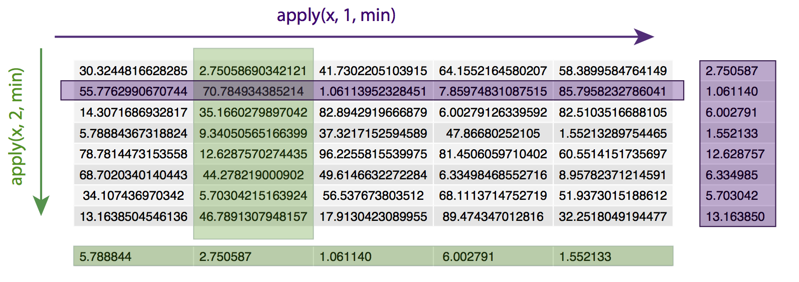
apply() loops over a data frame or matrix, applying the specified function to every row (specified by ‘1’) or column (specified by ‘2’). For example, given a matrix x, apply(x, 1, min) will apply the min() function to every row of the matrix x, returning the minimum value of each row. Similarly, apply(x, 2, min) will apply the min() function to every column of matrix x, returning the minimum value in each column.

# set a seed for consistency
set.seed(426)

# create a matrix
x <- matrix(runif(n=40, min=1, max=100), ncol=5)

# find the minimum value in each row
apply(x, 1, min)

# find the minimum value in each column
apply(x, 2, min)

Note: R is also very efficient at matrix operations. You can very easily and quickly apply simple operations to all the values of a matrix. For example, suppose you wanted to add a small value to every value in a matrix? Or divide all values in half

# Create a matrix
x <- matrix(runif(n=40, min=1, max=100), ncol=5)

# Examing the values in the matrix
x

# Add 1 to every value in the matrix
y <- x+1

# Divide all values by 2
z <- x/2

# Comfirm the effect
y
z

Functions in R

A function is a way to store a piece of code so we don’t have to type the same code repeatedly. Many existing functions are available in base R or the large number of packages available from CRAN and BioConductor. Occasionally however it may be helpful to define your own custom functions. Combining your own functions with the apply commands above is a powerful way to complete complex or custom analysis on your biological data. For example, suppose we want to determine the number of values in a vector above some cutoff.

# Create a vector of 10 randomly generated values between 1 and 100
vec <- runif(n=10, min=1, max=100)

# Create a function to determine the number of values in a vector greater than some cutoff
myfun <- function(x,cutoff){
 len <- length(which(x>cutoff))
 return(len)
}

# Run your the custom function on the vector with a cutoff of 50
myfun(vec,50)

# Create a matrix of 50 randomly generated values, arranged as 5 columns of 10 values
mat <- matrix(runif(n=50, min=1, max=100), ncol=5)

# Now, use the apply function, together with your custom function
# Determine the number of values above 50 in each row of the matrix
apply(mat, 1, myfun, 50)

Basic control structures

In general, it is preferable to “vectorize” your R code wherever possible. Using functions which take vector arguments will greatly speed up your R code. Under the hood, these “vector” functions are generally written in compiled languages such as C++, FORTRAN, etc. and the corresponding R functions are just wrappers. These functions are much faster when applied over a vector of elements because the compiled code is taking care of the low level processes, such as allocating memory rather than forcing R to do it. There are cases when it is impossible to “vectorize” your code. In such cases there are control structures to help out. Let’s take a look at the syntax of a for loop to sum a vector of elements and see how it compares to just running sum().

# install and load a benchmarking package
install.packages("microbenchmark")
library(microbenchmark)

# create a numeric vector to sum
x <- c(2, 4, 6, 8, 10)

# write a function to sum all numbers
mySum <- function(x){

    if(!is.numeric(x)){
        stop("non-numeric argument")
    }

	y <- 0
	for(i in 1:length(x)){
		y <- x[i] + y
	}

	return(y)
}

# both functions produce the correct answer
mySum(x)
sum(x)

# run benchmark tests
microbenchmark(mySum(x), sum(x), times = 1000L)

In mySum(), we use a for loop to sum all the elements of the vector. The syntax is fairly straightforward. We loop over the length of the argument passed to x and designate i as the variable to store the iteration of the loop. Prior to that, we use an if statement to make sure the user has supplied only numeric values. This statement simply executes the block of code in curly brackets. If the expression in parenthesis is TRUE, we use an ! to reverse the outcome of the result given by is.numeric(). All of this is defined as a function. These benchmark tests show that sum() is 2-3 orders of magnitude faster than our handwritten mySum() function.

Overview of less common operators in R

As in any language R has all of the basic operators available +, -, &, | etc. There are a few operators however that you will occassionally see that are not so familiar. For exmaple you might have noticed the use of :: in the bioconductor section above. While we won’t get into a discussion of all of the operators available in R let’s go over a few that are commonly seen.

• :: Takes the syntax library::function and allows one to call an exported function from an installed R library without having to load the library.
• ::: Similar to above but allows one to call a function from an installed R library that is not exported and generally available to users.
• %in% The % signs denote a special operator which take arguments on both the left and right side of the operator. In this example %in% will find element in a vector on the left hand side of the operator which are also present on the right hand side. This is intended to make the code slightly easier to read.
• $ Provides a way to access components of an S3 object, commonly seen applied to data frames which will be discussed a bit later.
• @ Provides a way to access slots in an S4 object, package authors should in theory provider functions to access slots however this is not always the case.
• %>% While not part of a base R install the magrittr operator from the magrittr package provides the functionality of a pipe in R. It is intended to make code more readable instead of nesting functions whithin each other.
• ` While perhaps not an operator the backtick provides a way to use an operation that would otherwise be illegal R syntax. You might see this if a data frame column has a space for example.

With the explanations out of the way let’s see these operators in practice. Start by installing the lubridate package which just makes working with dates easier.

# Install the lubridate package
install.packages("lubridate")

# call a lubridate function without loading the library
leap_year(2008)
lubridate::leap_year(2008)

# Examine a function not exported by the package, (calling a function without parenthesis will print the source code)
check_period
lubridate::check_period
lubridate:::check_period

# example of the include operation
cancer_genes = c("BRAF","TP53","PTEN","BRCA1","MYC")
de_genes = c("GAPDH","NADPH","PTEN","ACTN","TP53","ALDH2")
de_genes %in% cancer_genes
de_genes[de_genes %in% cancer_genes]

# access a compnent of an object
g <- list(name = "braf", variant = "v600e")
g$name
g$variant

# Load the lubridate function
library(lubridate)

# access a component of an object
span <- interval(ymd_hms("2008-11-02 01:30:03"), ymd_hms("2010-12-25 07:35:15"))
period <- as.period(span)
period@year
period@month

# pipe to a function
install.packages("magrittr")
library(magrittr)
mtcars %>% head
head(mtcars)

# using backticks for illegal operations
data <- data.frame(gene=c("EGFR","ERBB2","ERBB3"), exon_count=c(12,13,11), length=c(2244,2541,1976))
names(data)[1]="gene name"
data$exon_count
data$gene name
data$`gene name`

Optional Practical Exercise (Advanced)

First, download an existing pre-processed and normalized gene expression dataset (right-click and save as). This dataset represents the GCRMA normalized data for 12030 probesets (Affymetrix U133A) from 189 Estrogen Receptor (ER) positive breast cancers. It includes Affymetrix probeset id, Entrez Gene ID, and Gene Symbol in addition to 189 expression values per probeset (row).

Using the skills you’ve learned above:

1. Read the file into R;
2. Extract a matrix of just the expression data values (probeset vs. sample) without the probe and gene ID columns;
3. Convert the log2 values to raw (unlogged) expression values;
4. Write custom functions to determine, for a vector, (A) the % of values with raw intensity >= 100 AND (B) the coefficient of variation;
5. Apply your custom functions to all the rows (probesets) of the expression matrix, save as separate vectors (optionally add to the imported data frame);
6. Extract the subset of the matrix for which (A) the % of values with raw intensity of at least 100 is >= 20 AND (B) the COV >= 0.7;

How many probesets pass the filtering criteria above?

Additional resources

• http://www.noamross.net/blog/2014/4/16/vectorization-in-r–why.html