Introduction to COSMIC

« Introduction to ProteinPaint Course Using R for Genomic Data Visualization and Interpretation »

COSMIC, the Catalogue Of Somatic Mutations In Cancer, hosted by the Wellcome Trust Sanger Institute, is one of the largest and most comprehensive resources for exploring the impact of somatic mutations in human cancer. It is the product of a massive expert data curation effort, presenting data from thousands of publications and many important large scale cancer genomics datasets. COSMIC acts as the main portal for at least four important projects or resources: COSMIC - the Catalogue Of Somatic Mutations In Cancer, the Cancer Gene Census, the Cell Lines Project and COSMIC-3D. Academic users can use and download (with registration) the data for free, so long as they do not re-distribute the data, and agree to the license terms. For-profit users must pay a fee to download COSMIC. These resources provide access to a very rich set of data, visualizations, and interpretations for understanding cancer mutations and cancer genes.

The COSMIC database

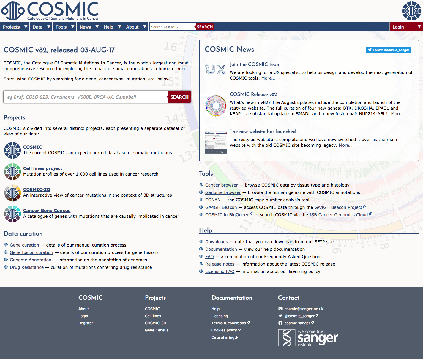
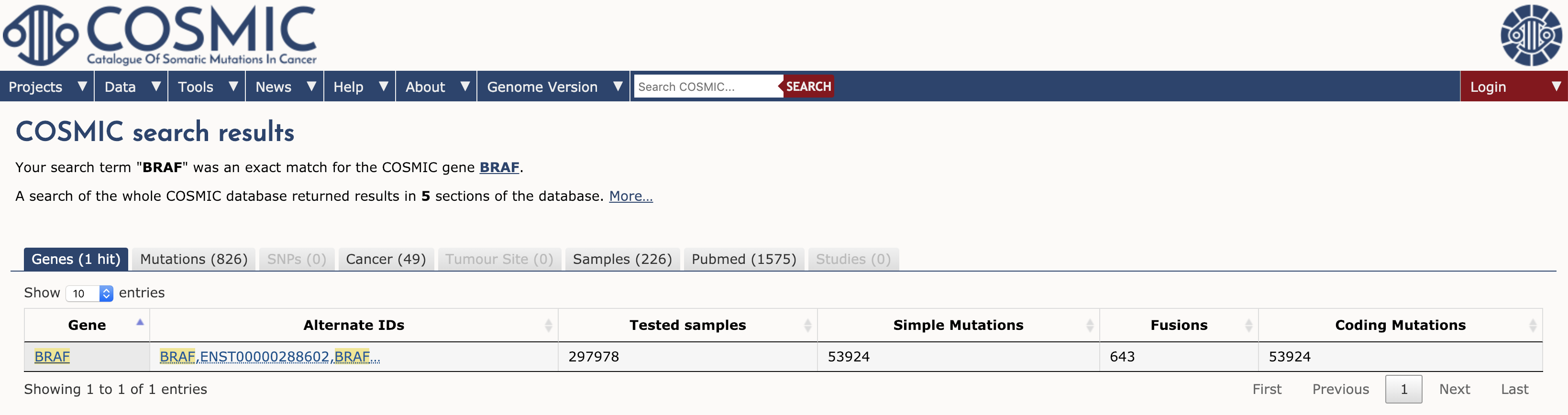
To browse COSMIC you can simply navigate to the main page and search for a gene, cancer type, mutation, etc in the search box. To illustrate we will explore the results for a single gene. Type BRAF in the search interface and hit enter. At the time of writing, this search term returned results for 1 gene, 826 mutations, 49 cancers, 226 samples, 1575 Pubmed citations, and 0 studies (see results tabs). Note that COSMIC contains results for almost 300,000 tested samples and over 50,000 mutations in BRAF.

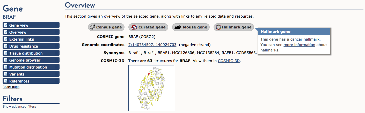
If we select the BRAF result, COSMIC returns a detailed page that provides: gene summaries, links to other COSMIC resources (e.g., Census genes, Hallmark genes, etc), external links, drug resistance, tissue distribution, genome browser view, mutation distribution, variants, and references. We will look at few of these sections. First, let’s look at the Overview section. Along the top of this section there are several useful icons. The ‘Census gene’ icon tells us that BRAF is a known cancer gene according to the Gene Census (see below). The next three icons tell us that it is also an ‘Expert curated gene’, that mouse insertional mutagenesis experiments support that BRAF is a cancer gene, and finally that BRAF is a ‘Cancer Hallmark’ gene. After these icons are many more details about BRAF including coordinates, synonyms, link to COSMIC-3D (see below), and more.

Next, let’s examine the Gene view. The histogram of mutation (substitution) frequency shows a very dramatic “hotspot” of mutations at position 600 (e.g., p.V600E). Mouse over this part of the histogram to see details. This is a very well-known driver mutation in multiple types of cancer.

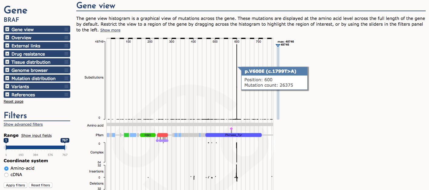
What part (domain) of the BRAF protein is affected by the p.V600E mutation?

The protein tyrosine kinase domain (Pfam)

Finally, navigate to the ‘Tissue distribution’ section. Sort the table by ‘Point mutations’ -> ‘% Mutated’. Notice that cancers of the thyroid and skin (e.g., melanoma) are by far the most consistently mutated at the BRAF gene locus (note NS means not specified). A subset of samples also display copy number variation (CNV) gains and up-regulated expression. In general certain predominanly mutated genes tend to be associated with cancers of certain origins. However, there are many exceptions to this statement and some genes (e.g., TP53) are widely mutated in many different cancer types.

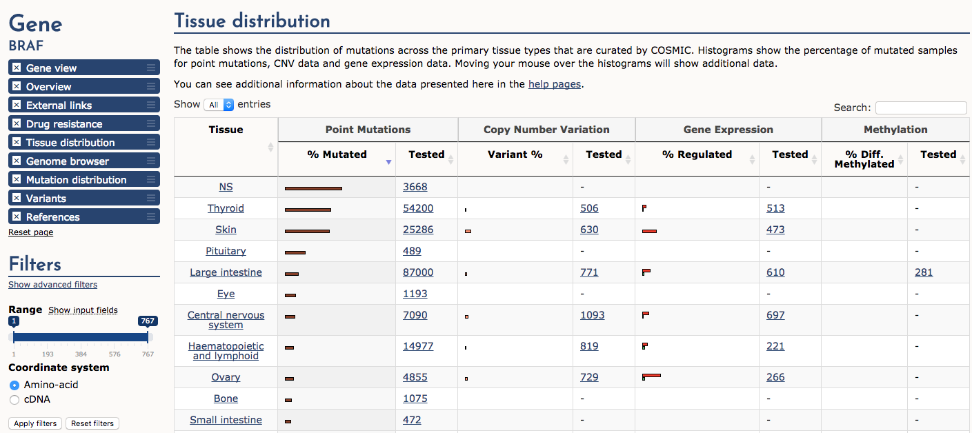
What cancer tissue type is most commonly affected by BRAF over-expression?

Approximately 15% of ovarian cancers are affected by BRAF over-expression

The Cancer Gene Census

The Cancer Gene Census (CGC) is an ongoing effort to catalogue those genes for which mutations (somatic or germline) have been causally implicated in cancer. The original census and analysis was published in Nature Reviews Cancer by Futreal et al. 2004 but it continues to receive regular updates. The CGC is widely regarded as a definitive list of cancer genes (tumor suppressors and oncogenes). Navigate to the Cancer Gene Census from the dropdown ‘Projects’ menu available on any COSMIC page. This page is broken into three main sections: Cancer Gene Census, Breakdown, and Abbreviations. In the first section, a simple table of all Cancer Gene Census genes is displayed.

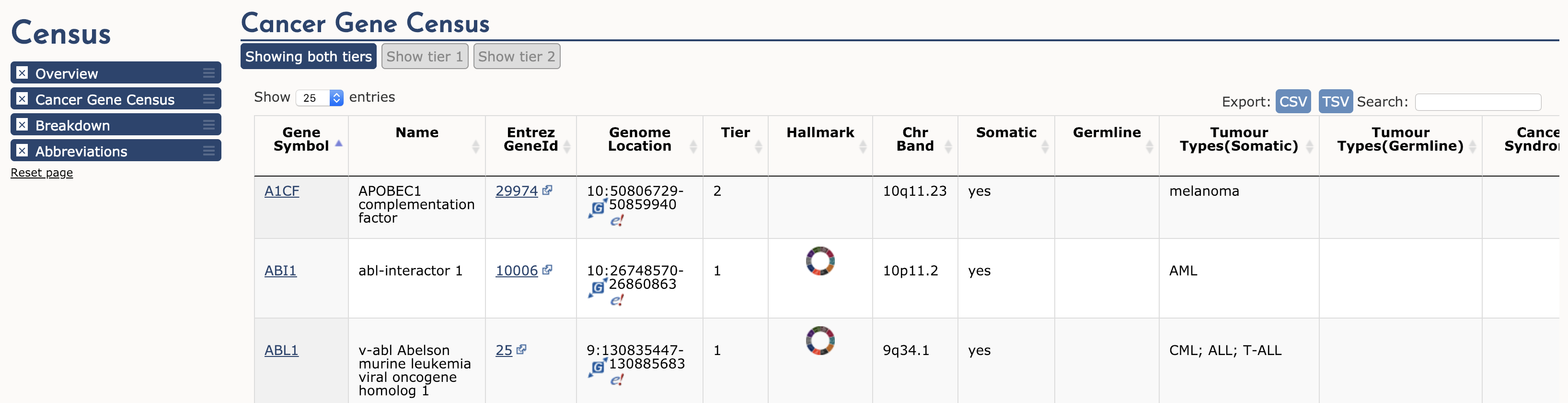
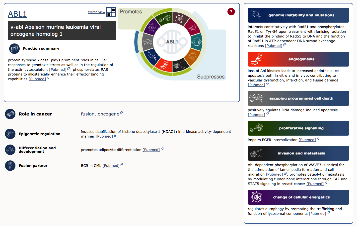
To illustrate, lets examine ABL1 (the third gene in the table). The first four columns provide the gene’s descriptive name, links to its COSMIC and Entrez gene pages, and genomic region with links to COSMIC and Ensembl Browser views. Other columns tell us that ABL1 is located on chromosome band 9q34.1, known to be somatically mutated in CML, ALL, and T-ALL. It acts as an oncogene and as a gene fusion partner. In fact, ABL1 is one part of perhaps the most famous cancer fusion, BCR-ABL, the product of the Philadelphia chromosome rearrangement. This fusion defines and drives nearly all cases of CML, and its discovery lead to one of the most successful examples of targeted therapy (Imatinib). To learn more about ABL1’s role in cancer select the ‘Census Hallmark’ icon. A ‘Hallmark’ is a reference to the seminal paper by Hanahan and Weinberg (2000), updated in 2011, in which they proposed that all cancers share six (now ten) common traits (hallmarks) that explain the transformation of normal cells into malignant cancer cells. Cancer Gene Census curators have attemped to assign each cancer gene in the census to one or more of these Hallmarks. The graphic shows which hallmarks are promoted (green bars) or suppressed (blue bars) by ABL1. In this case, ABL1 is thought to promote proliferative signalling, change of cellular energetics, genome instability, angiogenesis, invasion and metastasis, and suppress programmed cell death.

How many tumor supressor genes (TSGs) and oncogenes are there in CGC?

At time of writing there were 315 TSGs and 315 oncogenes in the CGC. Interestingly, there are 72 genes that function as both oncogene and TSG.

Note: You will need to register with COSMIC to download the complete Cancer Gene Census. You could then load this file in R, and use linux commandline, or some other approach to determine the list of TSGs and oncogenes currently documented in the CGC.

« Introduction to ProteinPaint Course Using R for Genomic Data Visualization and Interpretation »

Introduction to ProteinPaint

« Introduction to liftover tools Course Introduction to COSMIC »

ProteinPaint is a tool made available as part of the PeCan Data Portal. The principle goal of this data portal is to facilitate exploration of childhood cancer genomics data. However, some tools, such as ProteinPaint are generally useful for visualizing the recurrence of any set of variants in a gene in the context of protein domains and other information.

This section will provide a brief introduction to ProteinPaint’s features and demonstrate its use with a few examples and exercises.

The tool is entirely web based. First navigate to the tool’s homepage: ProteinPaint. Note that it has its own tutorials.

Guided tour of pre-loaded data

Go through the following exercise to explore the functionality of this resource:

Choose an example gene to explore (e.g. EGFR). Enter it in the search box and select it from the drop down of suggestions.

Select the gene name (top left) to view a summary of the gene.
Use the CONFIG option (right side) to change between display modes by selecting switch display mode. Try the Splicing RNA option. Note these options are also available from the gene summary view mentioned above.

Use the Tracks button to view the list of available tracks and turn on the RefGene track.

Use the CONFIG menu to change switch display mode back to Protein. Also turn off the RefGene track.
Select pre-loaded data to display (Pediatric, COSMIC, and ClinVar). Select COSMIC for this example. Use the ABOUT popup to learn more about each data source.
Zoom In on a mutation hotspot and navigate around that region. Once done, Zoom Out x50 to return to a view of the entire gene.

Under the More menu, try Select a region to highlight. Select a region containing a hotspot mutation. Change the highlight color using the same menu.

Clear the highlighted region. Now use the + add protein domain button (bottom left) to add a custom domain of interest. e.g. MUTATION HOTSPOT ; 700 900; red

Mouse over the gene diagram to view details on individual domains and amino acid positions.
Select specific variants to learn more about what diseases they occur in. For example, load ERBB2 and the COSMIC data track. Two of the most common mutations are S310F and L755S. Select both of these. Which is more common in breast cancer? Use the List option to learn more about individual variant observations.

Importing custom data

Suppose we want to load a custom data set of our own variants into ProteinPaint. For illustration, we will use CIViCs list of VHL variants. To get that list go to www.civicdb.org, select SEARCH, select the Variants tab, create a query where Gene is VHL, and hit the Search button. Once the query completes, use the Get Data option to Download CSV. Save this file. Rename it to CIViC-VHL-Variants.csv. We’ll need to reformat the data before inporting it into ProteinPaint.
Open this file in R and perform the clean-up as follows:

# Load the data downloaded from CIViC
setwd("~/Downloads/")
dir()
x = read.csv(file = "CIViC-VHL-Variants.csv", as.is=1:4)

# Store only the variant names that we will parse for protein coordinates
vhl_variants1 = x[,2] 

# Tidy up the names to remove the c. notations
vhl_variants2 = gsub("\\s+\\(.*\\)", "", vhl_variants1, perl=TRUE)

# Remove complex expressions beyond the "fs" in some variants
vhl_variants3 = gsub("fs.*", "fs", vhl_variants2, perl=TRUE)

# Limit to only those variants with a format like: L184P
vhl_variants4 = vhl_variants3[grep("^\\w+\\d+\\w+$", vhl_variants3, ignore.case = TRUE, perl=TRUE)]

# Remove variants with an underscore
vhl_variants5 = vhl_variants4[grep("_", vhl_variants4, ignore.case = TRUE, perl=TRUE, invert = TRUE)]

# Store the variant names for later
vhl_variant_names = vhl_variants5

# Extract the amino acid position numbers
vhl_variant_positions = gsub("\\D+(\\d+)\\D+", "\\1", vhl_variants5, perl=TRUE)

# Create a variant types list
# M=MISSENSE, N=NONSENSE, F=FRAMESHIFT, I=PROTEININS, D=PROTEINDEL, S=SILENT
types = vector(mode = "character", length = length(vhl_variant_names))
types[1:length(vhl_variant_names)] = "M"
types[grep("\\*", vhl_variant_names, ignore.case = TRUE, perl=TRUE)] = "N"
types[grep("fs", vhl_variant_names, ignore.case = TRUE, perl=TRUE)] = "F"
types[grep("ins", vhl_variant_names, ignore.case = TRUE, perl=TRUE)] = "I"
types[grep("del", vhl_variant_names, ignore.case = TRUE, perl=TRUE)] = "D"

# Store the values we care about in a new data frame
vhl_variants_final = data.frame(vhl_variant_names, vhl_variant_positions, types)
head(vhl_variants_final)

# Create the final format strings requested for ProteinPaint of the form: R200W;200;M
format_string = function(x){
  t = paste (x["vhl_variant_names"], x["vhl_variant_positions"], x["types"], sep = ";")  
  return(t)
}
output = apply(vhl_variants_final, 1, format_string)

# Write the output to a file
write(output, file="CIViC-VHL-Variants.formatted.csv")

Open the resulting file (CIViC-VHL-Variants.formatted.csv) in a text editor.
Then, in ProteinPaint load the VHL gene.
Use the + button to add data (top center), and choose the SNV/Indel option.
Then paste the formatted variant lines from the R cleanup exercise into that box and hit submit.

Compare the VHL variants from CIViC to those in ClinVar.

ProteinPaint practice exercises

What are the three most recurrent mutation in PIK3CA according to COSMIC?

Get a hint!

Load PIK3CA, activate the COSMIC track, and look for the mutations with highest patient counts

Answer

H1047R, E545K, and E542K are the most recurrent mutations in PIK3CA according to COSMIC

What is the top tissue of origin observed for each of these three mutations?

Get a hint!

Click on the circle for each mutation and examine the tissue distribution plot

Answer

H1047R (breast), E545K (large intestine), and E542K (large intestine)

Load the Pediatric data for RUNX1T1. (A) What special kind of variant is indicated? (B) Load the RNA-seq plot for these data. Mouse over the RUNX1 variant. What interesting pattern do you observe? (C) Highlight the top 25 samples in the RNA-seq expression plot. What type of cancer dominates?

Get a hint!

Load RUNX1T1, make sure the Pediatric data track is activated, and make sure the RNA-seq gene expression panel is open

Answer

(A) RNA gene fusion variants. (B) The RUNX1-RUNX1T1 (aka AML-ETO) fusion variant corresponds to samples with very high RUNX1T1 expression. (C) AML cancer dominates the top 25 samples with highest RUNX1T1 expression.

Repeat the exercise above where we extract variants from CIViC for KRAS, create a clean version of these data, and load them into ProteinPaint.

Get a hint!

You should be able to do almost exactly what we did with VHL, but for KRAS instead

Advanced exercise. Identify a set of variants from your own gene for a single gene. Repeat the exercise above using these variants. If they are not human variants, it may be possible to first identify the closest human ortholog, and second to do “lift over”” of the coordinates.

Get a hint!

Depending on the form of the variants, some different kind of parsing and reformatting may be needed. If you need to convert the variants from one species to another you will learn more about tools for identifying orthologs and performing liftovers in later sections of this workshop. You may want to come back to this exercise...

« Introduction to liftover tools Course Introduction to COSMIC »

Posts

Genomic Visualization and Interpretations

Introduction to COSMIC

The COSMIC database

The Cancer Gene Census

Genomic Visualization and Interpretations

Introduction to ProteinPaint

Guided tour of pre-loaded data

Importing custom data

ProteinPaint practice exercises

Introduction to COSMIC

Introduction to ProteinPaint