Welcome to the blog

Posts

My thoughts and ideas

Genome Browsing and Visualization - Ensembl | Griffith Lab

Genomic Visualization and Interpretations

Genome Browsing and Visualization - Ensembl

The Ensembl Genome Browser provides a portal to sequence data, gene annotations/predictions, and other types of data hosted in the various Ensembl databases. Many consider Ensembl to be the most comprehensive and systematic gene annotation resource in the world. Ensembl supports a large number of species and makes data available through a powerful web portal as well as through direct database downloads and APIs. Their excellent Help & Documentation pages provide instruction on using the website, data access, APIs, and their procedures for gene annotation and prediction. Their outreach team have put together extensive teaching materials that are available for free online. Rather than duplicate effort, we have linked to some of their instructional videos below. We will review these and then perform some simple exercises to familiarize ourselves with the Ensembl Genome browser.

Introduction to genome browsers using Ensembl


What is a scaffold?

A scaffold is a long stretch of genomic sequence that has been assembled but not necessarily yet assigned to a chromosome. A scaffold is typically made up of contigs and gaps assembled into a single sequence with known order and orientation between the contigs.

Does Ensembl produce its own genome assembly?

No. Ensembl imports genome assemblies from other sources (e.g., the Genome Reference Consortium) and then annotates genes and other features to the same reference as available elsewhere (UCSC, NCBI, etc).

When do transcripts belong to the same gene?

Transcripts that share exons transcribed from the same strand are considered to belong to the same gene locus in Ensembl.

What are the two main types of transcripts annotated in Ensembl?

The two main types of transcripts annotated in Ensembl are (protein) coding and non-coding.


The Ensembl Genome Browser: an overview


What is a stable identifier in Ensembl?

Stable identifiers are IDs for features (gene, transcript, protein, exon, etc.) that should not change even when underlying data and meta-data for those features change. Examples include ENSG..., ENST..., ENSP... for human Ensembl gene, transcript, and proteins. Other species will have modified prefixes but follow the same conventions. For example, Ensembl dog genes are named ENSCAFG...

How many protein coding transcripts does human CDKN2B have?

Ensembl has two protein coding transcripts annotated for human CDKN2B.

Which species has a CDKN2B orthologous gene that most closely matches human?

The Chimpanzee CDKN2B is 100.00 similar to its human counterpart. This can be determined under the Comparative Genomics Gene Tree or Orthologues section of the human CDKN2B gene page.


Data Visualization with Ensembl

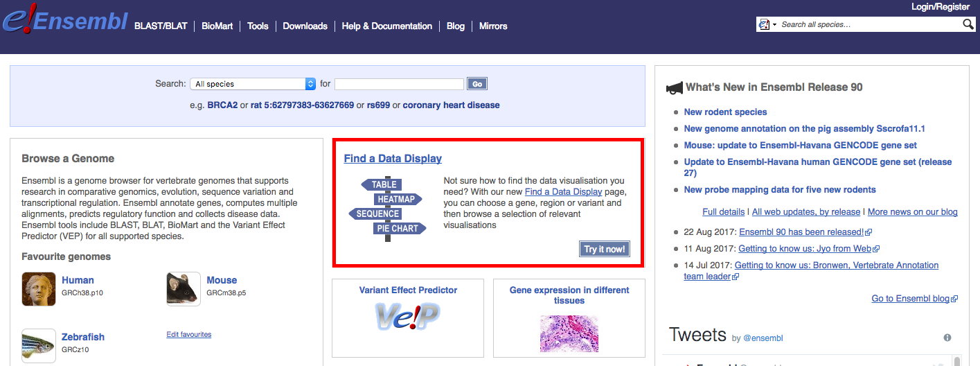
An excellent way to explore the data visualization possibilities with Ensembl is to use their Find a Data Display page. This is linked directly from the Ensembl home page (see red box below). From this page, you can you can choose a gene, region or variant and then browse a selection of relevant visualisations.

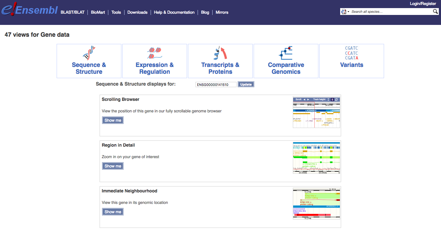
Navigate to the Find a Data Display page. To illustrate, select ‘Species’ -> ‘Human’, ‘Feature Type’ -> ‘Genes’, and then ‘Identifier’ -> ‘TP53’. You will be presented with a number of possible matches. Select the exact ‘TP53’ match and select ‘Go’. The results page, at time of writing, returned a comprehensive set of 47 views for TP53 (ENSG00000141510) associated with: Sequence & Structure, Expression & Regulation, Transcripts & Proteins, Comparative Genomics, and Variants. We will display just a few examples here and then explore others through exercises.

Select the ‘Splice Variants’ view and scroll down the page a little. You will see a graphical representation (see below) of all known and predicted transcripts for TP53, and how these exons line up with each other and with other features such as protein domains.


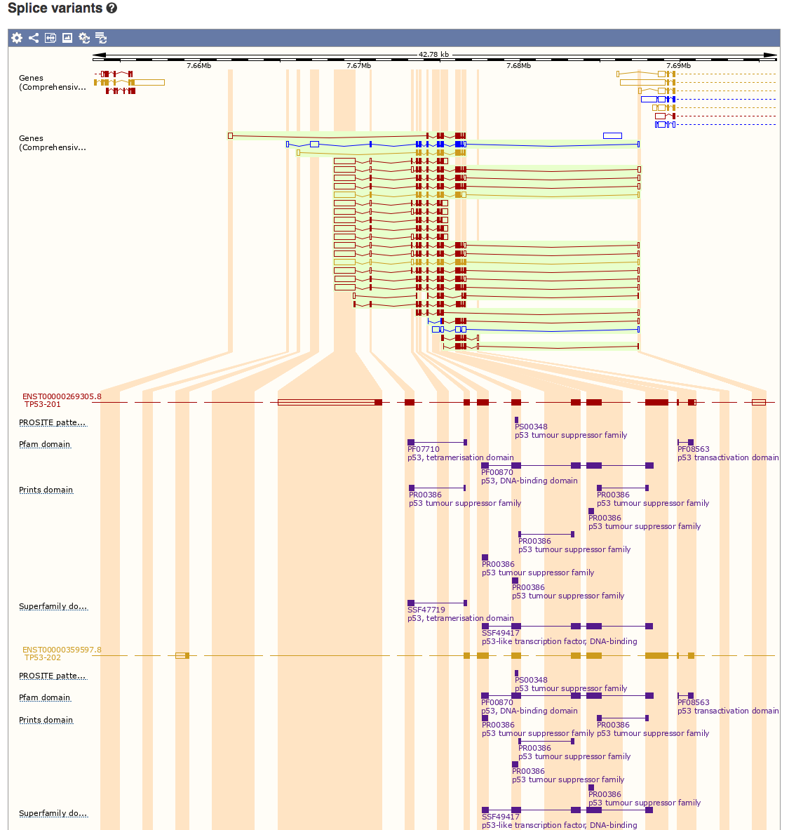
How many different protein domains are annotated for TP53 according to the Pfam database?

Pfam reports three domains for TP53: tetramerisation, DNA-binding, and transactivation domains.

Which domain is most consistently conserved across the many different isoforms of TP53?

It appears that all or part of the DNA-binding domain is the most consistently conserved across the isoforms of TP53 based solely on which exons are included in each isoform.


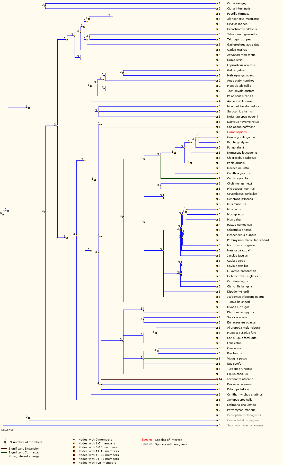
Next, examine the ‘Gene Gain/Loss Tree’ for TP53. User your browser back button (or the instructions above) to go back to the data display views for TP53 and then select ‘Gene Gain/Loss Tree’. If this does not work, you can also select ‘Gene Gain/Loss tree’ from the side bar of ‘Gene-based displays’ -> ‘Comparative Genomics’ menu on any gene page.


Which species has the most significant increase in TP53 gene?

The TP53 gene family has 14 members for elephant compared to 2, 3 or 4 for all other Ensembl species. In fact, a study in 2016 reported finding at least 20 copies of TP53 in the elephant genome and suggested that this explains why elephants do not have increased risk of cancer despite their larger body size.


Ensembl Data Display Exercise

Using your knowledge of tissue-specific expression for a specific species/gene, explore the Gene Expression views in Ensembl. Does the available data confirm your knowledge of these genes. For example, considering human genes, we might investigate: MSLN (Mesothelin) - normally present on the mesothelial cells lining the pleura, peritoneum and pericardium and over-expressed in several cancers. Other interesting human/cancer tissue markers include: KLK3 (PSA), EPCAM, SCGB2A2 (Mammaglobin), CD19, etc. Below you can see an example for PSA.


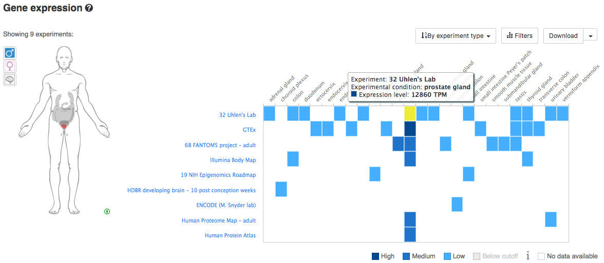
What is the tissue expession pattern for PSA?

PSA is expressly almost exclusively in the prostrate gland and only lowly in a few other tissues.


Ensembl Genomes - Extending Ensembl across the taxonomic space

The EnsemblGenomes site hosts genome-scale data from ~52,000 species, most of which are not available through the core Ensembl. Data are organized into five taxonomic categories: bacteria (n=50364), protists (n=200), fungi (n=1802), plants (n=63), and metazoa (n=74). Each generally provides at least a preliminary genome assembly, gene annotations, and to varying degrees includes: variation data, pan compara data, genome alignments, peptide alignments, and other alignments. If your species is not in Ensembl it is worth checking whether it is available in EnsemblGenomes.

Review of Central Concepts | Griffith Lab

Genomic Visualization and Interpretations

Review of Central Concepts

Before we proceed, it may be beneficial to review some central concepts and themes in the realm of genomics and computational biology. Here we provide a very brief overview of core tenets, and common “gotchas” for these disciplines, as they pertain to this course. We will also introduce the demonstration datasets used throughout the subsequent modules.


Central Dogma

Lets start with the core tenet of genomics, the central dogma:

“The Central Dogma. This states that once ‘information’ has passed into protein it cannot get out again. In more detail, the transfer of information from nucleic acid to nucleic acid, or from nucleic acid to protein may be possible, but transfer from protein to protein, or from protein to nucleic acid is impossible. Information means here the precise determination of sequence, either of bases in the nucleic acid or of amino acid residues in the protein.” –Francis Crick 1956

As quoted above, the central dogma describes the flow of biological information, encoded in deoxyribonucleic acid (DNA), ribonucleic acid (RNA) and protein. In essence it states that information cannot flow backward from a protein, that is to say transfer of information from a protein to RNA, DNA, or replicated by another protein is impossible. The general flow of information is through the copying of DNA by DNA replication, the creation of RNA from transcription of DNA, and the creation of proteins via translation of RNA. These processes occur in most cells and are considered mechanisms of general transfer. Special exceptions do exist in the form of RNA replication and reverse transcription however these processes are mostly limited to viruses.

Delving in a bit deeper, DNA takes the form of a double stranded helix comprised of pairs of complementary bases. Adenine (A) and Guanine (G) are classified as purines and complement the pyrimidines Thymine (T) and Cytosine (C) respectively. During transcription DNA is transcribed into a single stranded mRNA molecule in which T bases are converted to uracil (U) and RNA processing such as the removal of introns is performed. This results in a mature mRNA structure composed (for a protein-coding gene) of a 5’ UTR, Coding sequence (CDS), 3’ UTR, and a polyadenylated tail. The mature mRNA is then translated into a peptide sequence beginning at the AUG start codon within the CDS, continuing for each nucleotide triplet codons, until a stop codon occurs. The resulting peptide is often subsequently modified (e.g., phosphorylation of specific residues) and folded into a functional protein. Essentially all “omic” technologies and assays leverage these naturally occuring properties (e.g., DNA/RNA complementarity) and processes (e.g., DNA replication via polymerase). Interpretation of omic data would not be possible without the decades of work to characterize these products, sequence reference genomes (e.g., The Human Genome Project), establish databases of gene annotations, and so on.

What is the reverse complement of: TCGCATTCAGCGGCCATCAGCAGTAAACATCTTAAC?

GTT AAG ATG TTT ACT GCT GAT GGC CGC TGA ATG CGA

Does the resulting sequence contain an open reading frame (ORF)?

Yes. Look for an ATG in frame with a TGA, TAA or TAG, or see the next question for the ORF

What is the mRNA sequence of: ATG TTT ACT GCT GAT GGC CGC TGA?

AUG UUU ACU GCU GAU GGC CGC UGA

What is the translated peptide for the sequence in the previous question?

Met-Phe-Thr-Ala-Asp-Gly-Arg-Stop (Methionine-Phenylalanine-Threonine-Alanine-Aspartic acid-Glycine-Arginine-Stop)


Omic technologies and Data

The advent of rapid and cheap massively parallel sequencing has dramatically increased the availability of genome, transcriptome, and epigenome data. This revolution has given rise to a plethora of standardized (and non-standard) omic analysis workflows, file formats, and a deluge of sequence data. Extracting biologically meaningful conclusions from this data remains a principal challenge. In this course we will learn to visualize several types of omic data in a meaningful way.


Reference Files

Over this course we will be working with a number of reference/data files to aid in analysis and interpretation of our data. All of these files are in standardized formats and are freely available. A brief description of each reference file is given below.

What character designates a header in a fasta file?

">"

What character designates a Phred Q value of 30 (Sanger format)?

"?"

For a BAM alignment record, what does a CIGAR string of 60M1D40M signify?

This alignment has 60bp of matching sequence, a one bp deletion, and then an additional 40bp of matching sequence


Genomic annotation resources, browsers, etc.

A common task in genomic analysis and interpretation is collating sequence features or other information to visualize. For example you may have a genomic position and want to know if it is on a gene, the conservation at that position, etc. There are quite a few annotation resources available for this task. In this course we will focus on the ensembl variant effect predictor however a few other resources are listed below.

In the same vein, it is often beneficial to view your reference genome or actual sequence data, again there are many resources available for this, we’ll go over these within the course.


Common problems

Within computational biology there are a number of pitfalls that beginners can fall into. Here we review a few of the most common, to make life easier down the road.

Genomic coordinate systems

Within computational biology there are two competing coordinate systems for specifying regions within the genome. These two systems number either the nucleotides in the genome directly (1-based), or the gaps between nucleotides (0-based). Let’s look at the diagram below displaying an imaginary sequence on chromosome 1 to help illustrate this concept.

To indicate a single nucleotide variant:

To indicate insertions or deletions:

What is the difference between 0-based and 1-based coordinates?

0-based coordiantes number between nucleotides, 1-based coordinates number nucleotides directly.

Differences in carriage returns

In all unix based systems (OSX included) new line characters, commonly referred to as carriage returns are designated by the character “\n”. However this is not a universal standard, windows programs such as Excel designate a carriage return as “\r\n” mostly to maintain compatability with MS-DOS. This can create problems when attempting to use a file made via a windows application on a unix system. Specifically, attempting to view one of these types of files on a unix system will not interpret “\r\n” as a new line but rather as “^M”. This is something to be aware of but is fortunately easily remedied through any text processing language. Below you will find an example for fixing this file through perl via a command line.

perl -pi -e 's/\r\n|\n|\r/\n/g' FileToChange.txt

In essence the command above calls the perl regular expression engine and substitutes “\r\n” or “\n” or “\r” with “\n”, editing the file in place.

Genome builds

When doing any sort of bioinformatic analysis it is good to be aware of the reference assembly upon which your data is based. Each species has it’s own reference assembly representing the genome of that species, and each species specific assembly can have multiple versions as our understanding of the genome for each species improves. When comparing across data sets, especially in terms of genomic coordinates, reference assemblies should always match. We will cover all of this in more detail in the liftOver section.

A detailed discussion of some commonly used human reference genome builds can be found here.


Introduction to demonstration data sets

Throughout this course we will be working with and visualizing many different datasets. Below we provide a brief overview of each core data set and what type of visualizations we will create with them.