Genome Browsing and Visualization - IGV
It is often necessary to examine sequencing data aligned to specific regions of the genome in order to obtain a clearer picture of genomic events. One of the most popular tools for this is the Integrative Genomics Viewer. After this lab you should be able to perform the following tasks:
- Visualize a variety of genomic data
- Quickly navigate around the genome
- Visualize read alignments
- Validate SNP/SNV calls and structural re-arrangements by eye
Installing IGV
Java is necessary to run IGV, you can download the java runtime environment (JRE) for your operating system here. To determine if this step is necessary type java -version at a command prompt, if the program is not >= 1.7 you’ll need to upgrade it. IGV can be downloaded here. This tutorial will make use of IGV version 2.3 or later, we strongly recommend that you upgrade IGV if you have an older version installed.
Data Set for IGV
We will be using publicly available Illumina sequence data from the HCC1143 cell line. The HCC1143 cell line was generated from a 52 year old caucasian woman with breast cancer. Additional information on this cell line can be found here: (tumor, TNM stage IIA, grade 3, primary ductal carcinoma) and HCC1143/BL (matched normal EBV transformed lymphoblast cell line). Reads within these cell lines have been filtered to Chromosome 21: 19,000,000-20,000,000 in order to reduce file sizes.
Visualization Part 1: Getting familiar with IGV
We will be visualizing read alignments using IGV, a popular visualization tool for HTS data.
First, lets familiarize ourselves with it.
Load a Genome and some Data Tracks
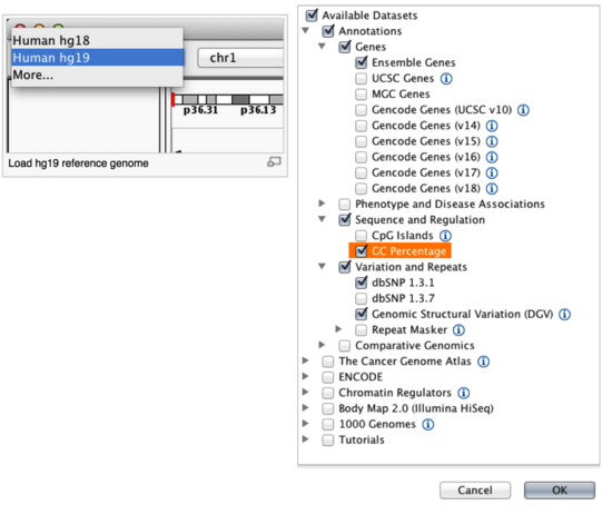
By default, IGV loads Human (hg19). If you work with another version of the human genome, or another organism altogether, you can change the genome by clicking the drop down menu in the upper-left. For this lab, we will be using Human (hg19).
We will also load additional tracks from the IGV Server using (File -> Load from Server...):
- Ensembl genes (or your favourite source of gene annotations)
- GC Percentage
- dbSNP 1.3.1 or 1.3.7
Load hg19 genome and additional data tracks
Navigation
You should see a listing of chromosomes for this reference genome. Choose 1, for chromosome 1.
Chromosome chooser

Navigate to chr1:10,000-11,000 by entering this into the location field (in the top-left corner of the interface) and clicking Go. This shows a window of chromosome 1 that is 1,000 base pairs wide and beginning at position 10,000.
Navigition using Location text field. Sequence displayed as thin coloured rectangles.
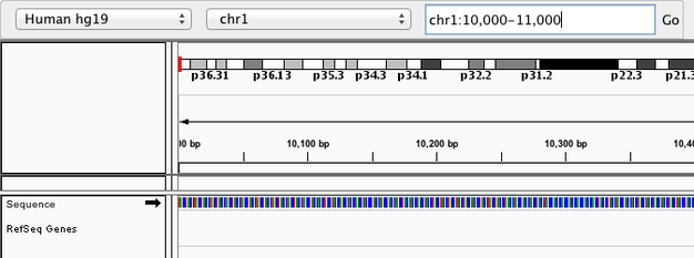
IGV displays the sequence of letters in a genome as a sequence of colours (e.g. A = green, C = blue, etc.). This makes repetitive sequences, like the ones found at the start of this region, easy to identify. Zoom in a bit more using the + button (top right) to see the individual bases of the reference genome sequence.
You can navigate to a gene of interest by typing it into the same box that the genomic coordinates are in and pressing Enter/Return. Try it for your favourite gene, or BRCA1 if you can not decide.
Gene model
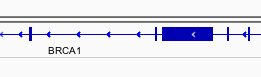
Genes are represented as lines and boxes. Lines represent intronic regions, and boxes represent exonic regions. The arrows indicate the direction/strand of transcription for the gene. When an exon box become narrower in height, this indicates a UTR.
When loaded, tracks are stacked on top of each other. You can identify which track is which by consulting the label to the left of each track.
Region Lists
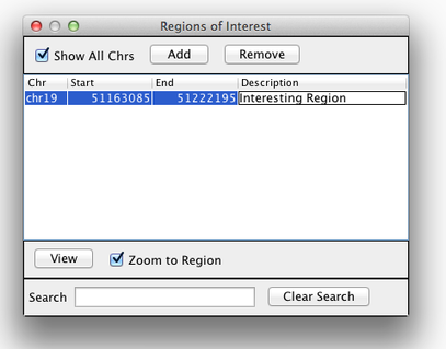
Sometimes, it is useful to save where you are, or to load regions of interest. For this purpose, there is a Region Navigator in IGV. To access it, click Regions > Region Navigator. While you browse around the genome, you can save some bookmarks by pressing the Add button at any time.
Bookmarks in IGV
Loading Read Alignments
We will be using the breast cancer cell line HCC1143 to visualize alignments. For speed, only a small portion of chr21 will be loaded (19M:20M).
HCC1143 Alignments to hg19:
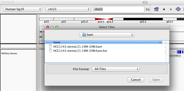
Copy the files to your local drive, and in IGV choose File > Load from File..., select the bam file, and click OK. Note that the bam and index files must be in the same directory for IGV to load these properly. Alternatively, you can copy the link location and load File > Load from URL....
Load BAM track from File
Visualizing read alignments
Navigate to a narrow window on chromosome 21: chr21:19,480,041-19,480,386.
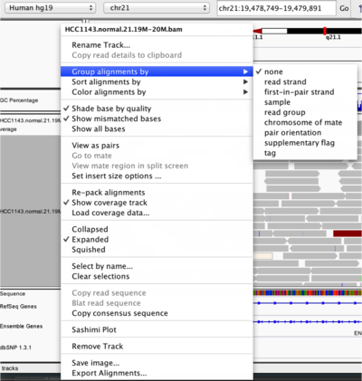
To start our exploration, right click on the track-name, and select the following options:
- Sort alignments by
start location - Group alignments by
pair orientation
Experiment with the various settings by right clicking the read alignment track and toggling the options. Think about which would be best for specific tasks (e.g. quality control, SNP calling, CNV finding).
Changing how read alignments are sorted, grouped, and colored
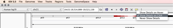
You will see reads represented by grey or white bars stacked on top of each other, where they were aligned to the reference genome. The reads are pointed to indicate their orientation (i.e. the strand on which they are mapped). Mouse over any read and notice that a lot of information is available. To toggle read display from hover to click, select the yellow box and change the setting.
Changing how read information is shown (i.e. on hover, click, never)
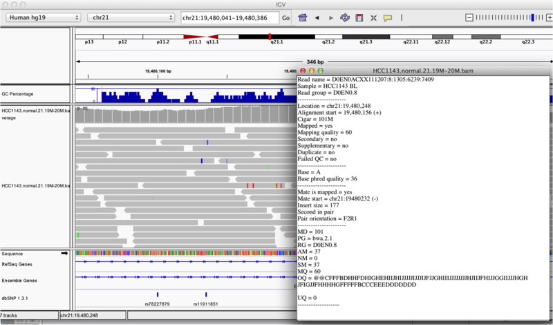
Once you select a read, you will learn what many of these metrics mean, and how to use them to assess the quality of your datasets. At each base that the read sequence mismatches the reference, the colour of the base represents the letter that exists in the read (using the same colour legend used for displaying the reference).
Viewing read information for a single aligned read
Visualization Part 2: Inspecting SNPs, SNVs, and SVs
In this section we will be looking in detail at 8 positions in the genome, and determining whether they represent real events or artifacts.
Two neighbouring SNPs
- Navigate to region
chr21:19,479,237-19,479,814 - Note two heterozygous variants, one corresponds to a known dbSNP (
G/Ton the right) the other does not (C/Ton the left) - Zoom in and center on the
C/TSNV on the left (chr21:19,479,321is the SNV position) - Sort alignments by
base - Color alignments by
read strand
Example1. Good quality SNVs/SNPs
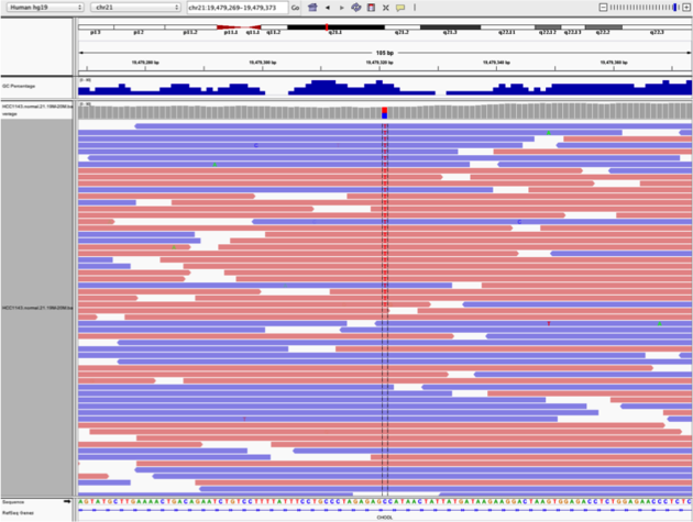
Notes:
- High base qualities in all reads except one (where the alt allele is the last base of the read)
- Good mapping quality of reads, no strand bias, allele frequency consistent with heterozygous mutation
What does Shade base by quality do?
This will change the opacity of the base in IGV based on how confident the sequencer was in calling that base using the phred score. This is beneficial in determining if a called variant is real or artifactual.
How does Color by read strand help?
Coloring by read strand will indicate if the DNA fragment sequenced was on the positive or negative strand. A variant occurring on only one strand could indicate an artifact.
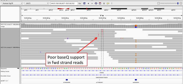
Homopolymer region with indel
Navigate to position chr21:19,518,412-19,518,497
Example 2a
- Group alignments by
read strand - Center on the
Awithin the homopolymer run (chr21:19,518,470), andSort alignments by->base
Example 2b
- Center on the one base deletion (
chr21:19,518,452), andSort alignments by->base
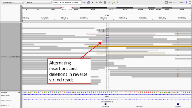
Notes:
- The alt allele is either a deletion or insertion of one or two
Ts - The remaining bases are mismatched, because the alignment is now out of sync
- The dpSNP entry at this location (rs74604068) is an A->T, and in all likelihood an artifact
- i.e. the common variants from dbSNP include some cases that are actually common misalignments caused by repeats
Coverage by GC
Navigate to position chr21:19,611,925-19,631,555. Note that the range contains areas where coverage drops to zero in a few places.
Example 3
- Use
Collapsedview - Use
Color alignments by->insert size and pair orientation - Load GC track
- See concordance of coverage with GC content
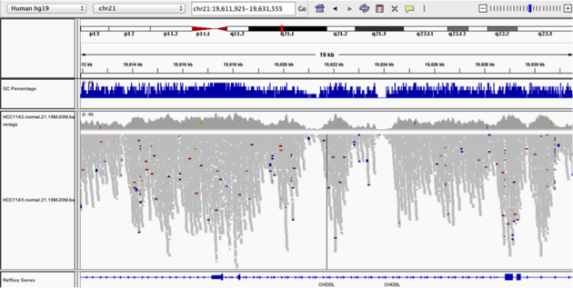
Why are there blue and red reads throughout the alignments?
The reads are colored by insert size, in paired data a blue read indicates the insert size is smaller than expected indicating a deletion. Conversely a red read indicates the insert size is larger than expected indicating an insertion.
Heterozygous SNPs on different alleles
Navigate to region chr21:19,666,833-19,667,007
Example 4
- Sort by base (at position
chr21:19,666,901)
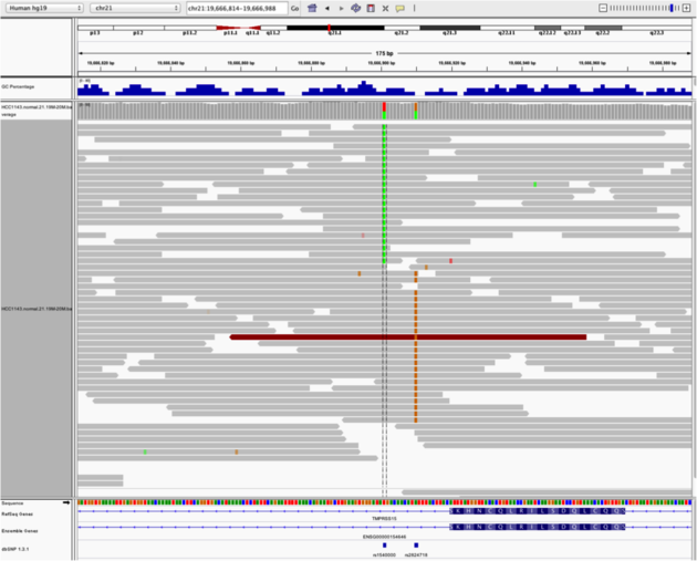
Note:
- There is no linkage between alleles for these two SNPs because reads covering both only contain one or the other
Low mapping quality
Navigate to region chr21:19,800,320-19,818,162
- Load repeat track (
File->Load from server...)
Load repeats
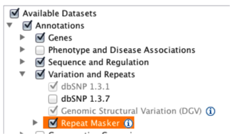
Example 5
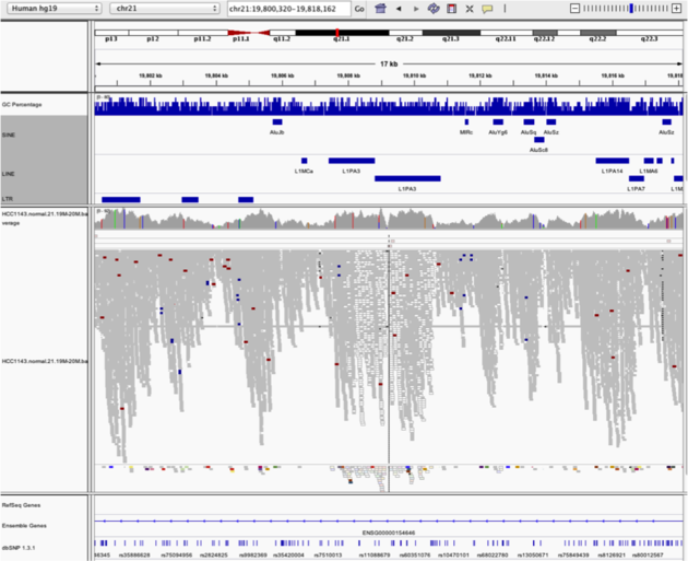
Notes:
- Mapping quality plunges in all reads (white instead of grey). Once we load repeat elements, we see that there are two LINE elements that cause this.
Homozygous deletion
Navigate to region chr21:19,324,469-19,331,468
Example 6
- Turn on
View as PairsandExpandedview - Use
Color alignments by->insert size and pair orientation - Sort reads by insert size
- Click on a red read pair to pull up information on alignments
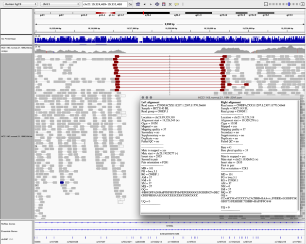
Notes:
- Typical insert size of read pair in the vicinity: 350bp
- Insert size of red read pairs: 2,875bp
- This corresponds to a homozygous deletion of 2.5kb
Mis-alignment
Navigate to region chr21:19,102,154-19,103,108
Example 7
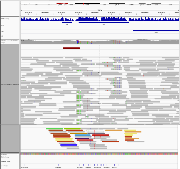
Notes:
- This is a position where AluY element causes mis-alignment.
- Misaligned reads have mismatches to the reference and well-aligned reads have partners on other chromosomes where additional ALuY elements are encoded.
- Zoom out until you can clearly see the contrast between the difficult alignment region (corresponding to an AluY) and regions with clean alignments on either side
Translocation
Navigate to region chr21:19,089,694-19,095,362
Example 8
- Expanded view
Group alignments by->pair orientationColor alignments by->pair orientation
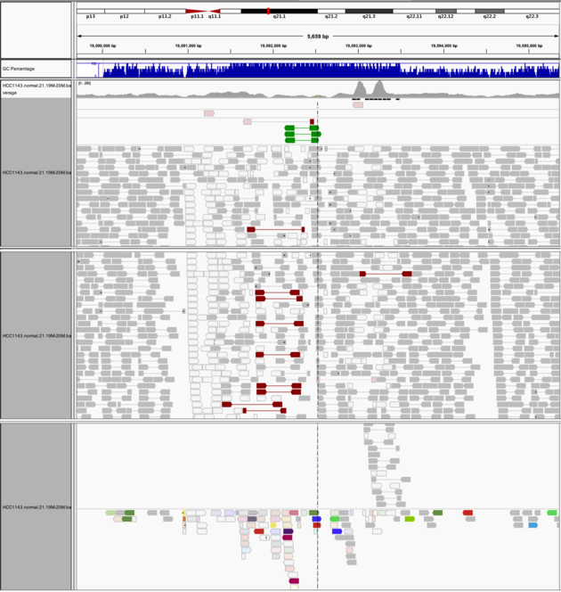
Notes:
- Many reads with mismatches to reference
- Read pairs in RL pattern (instead of LR pattern)
- Region is flanked by reads with poor mapping quality (white instead of grey)
- Presence of reads with pairs on other chromosomes (coloured reads at the bottom when scrolling down)
A Standard Operating Procedure (SOP) for Manual Review of Variants
As illustrated above, manual review of sequence alignments is often necessary to confirm/validate called variants. Despite the widespread usage of manual review, published studies rarely document the procedure and best practices for this review. To address this, Barnell et al published a “Standard operating procedure for somatic variant refinement of sequencing data with paired tumor and normal samples”. This SOP documents methods and examples of how to categorize variants into four different classes (Somatic, Germline, Ambiguous or Fail) with 19 tags for common sources of sequence or analysis artifacts. This SOP supports and enhances manual somatic variant detection by improving reviewer accuracy while reducing the inter-reviewer variability for variant calling and annotation.
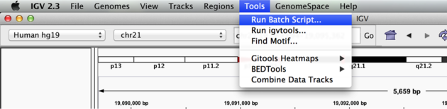
Visualization Part 3: Automating Tasks in IGV
We can use the Tools menu to invoke running a batch script. Batch scripts are described on the IGV website:
- Batch file requirements: http://software.broadinstitute.org/software/igv/batch
- Commands recognized in a batch script: http://software.broadinstitute.org/software/igv/PortCommands
- We also need to provide sample attribute file as described here: http://software.broadinstitute.org/software/igv/DisplayOptionsAttributes
Download the batch script and the attribute file for our dataset:
- Batch script: Run_batch_IGV_snapshots.txt
- Attribute file: Igv_HCC1143_attributes.txt
Now run the file from the Tools menu:
Automation
Notes:
- This script will navigate automatically to each location in the lab
- A screenshot will be taken and saved to the screenshots directory specified