Introduction to copy number frequency plots
A common task in any bioinformatic analysis of next generation sequencing data is the the determination of copy number gains and losses. The cnFreq() function from the GenVisR package is designed to provide a summary level view of copy number calls for a cohort of cases. It uses a barchart like plot to display the proportion or frequency of CN gains or losses observed across the genome. In this section we will use cnFreq() to explore the copy number frequencies and proportions for 10 her2 positive breast cancer samples from the manuscript “Genomic characterization of HER2-positive breast cancer and response to neoadjuvant trastuzumab and chemotherapy-results from the ACOSOG Z1041 (Alliance) trial.”
Loading data
The data we will be working with was generated with the R package Copycat2. The output of this program consists of a file containing segmented copy number calls. You can find these files on http://genomedata.org/gen-viz-workshop/GenVisR/, go ahead and download all files with a .cc2.tsv extension. Once these files are downloaded we will need to read them into R and coerce them into a single data frame with column names “chromosome”, “start”, “end”, “segmean”, and “sample”. As a first step install and load the stringr package we’ll need this to make some of the string manipulation we’ll be doing easier. Once stringr is loaded run through the rest of the R code below, we’ll explain step by step what’s going on in the paragraph below.
# load extra libraries
# install.packages("stringr")
library("stringr")

# get locations of all cn files
files <- Sys.glob("~/Desktop/*cc2.tsv")

# create function to read in and format data
a <- function(x){
    # read data and set column names
    data <- read.delim(x, header=FALSE)
    colnames(data) <- c("chromosome", "start", "end", "probes", "segmean")

    # get the sample name from the file path
    sampleName <- str_extract(x, "H_OM.+cc2")
    sampleName <- gsub(".cc2", "", sampleName)
    data$sample <- sampleName

    # return the data
    return(data)
}

# run the anonymous function defined above
cnData <- lapply(files, a)

# turn the list of data frames into a single data frame
cnData <- do.call("rbind", cnData)
After the stringr package is loaded we need to create a vector of all copy number files we downloaded, for this we use the function Sys.glob(). Once we have our vector of copy number files we can create an anonymous function, a, to read data into R from a file path. In this function we first use read.delim() to read in our data, remember to set the parameter header=F as these files have no header. With the file read in as a data frame we can then use the function colnames() to set the appropriate column names. All of the required column names are already present save for one, the sample name. We use the str_extract() function from the stringr package along with a call to gsub() to pull this information from the file name and add this as another column. We use the lapply() function to run the anonymous function we defined on each file path giving us a list of data frames with copy number data read in. Finally we use the function do.call() to execute the function rbind() each data frame in the list giving us a single data frame of copy number values.
Creating an initial plot
Now that we have our copy number calls loaded into R we can call the cnFreq() on our data set. We will also need to give a genome assembly via the parameter genome. This expects a character string specifying one of “mm9”, “mm10”, “hg19”, “hg38”, and “rn5” and is used to ensure that the entire chromosomes for the genome is plotted. In the next version of GenVisR this function will be expanded to allow input of custom genome boundaries if needed.
# call the cnFreq function
cnFreq(cnData, genome="hg19")
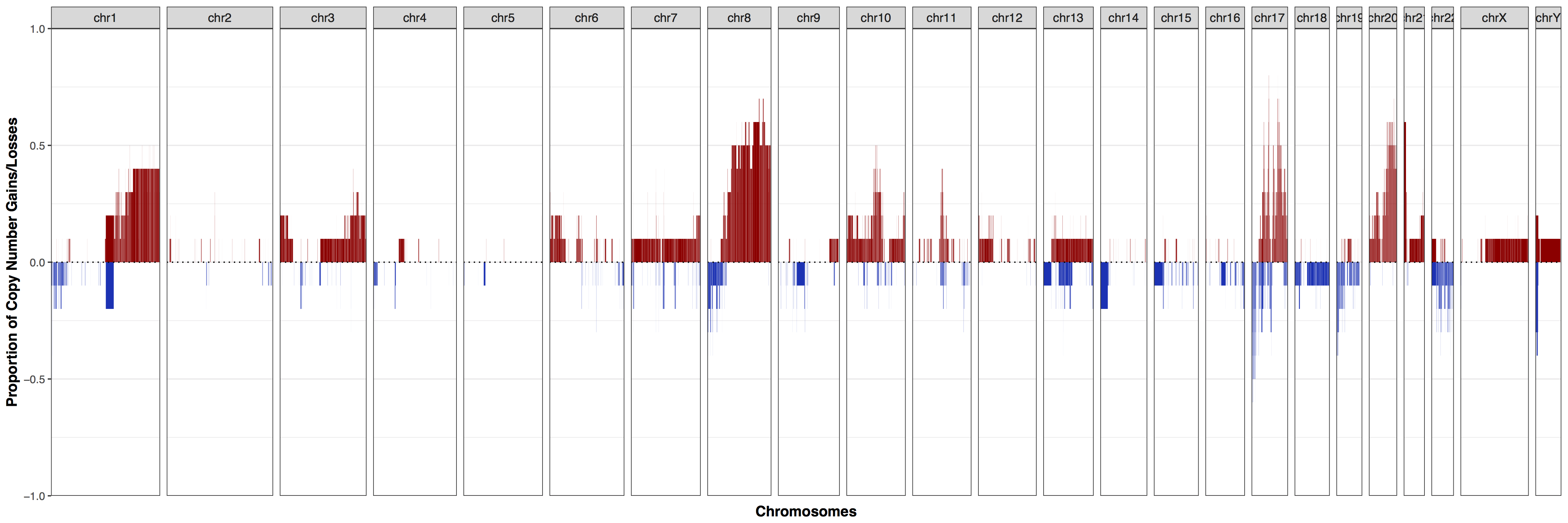
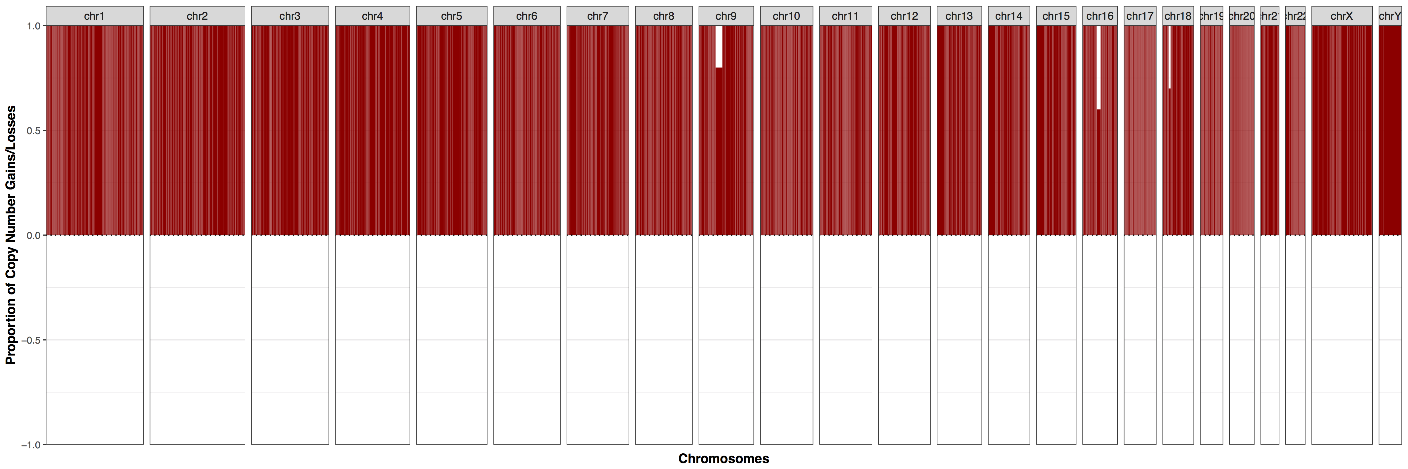
As we can see from the plot above our cohort exhibits a strong amplification signal across much of the genome, particularly chromosomes 8, 17, and 20 where over half of samples have some sort of copy number gain. You might be asking what in cnFreq() constitutes as a copy number gain or loss. This is controlled with the parameters CN_low_cutoff and CN_high_cutoff with calls ≤ 1.5 and ≥ 2.5 being evaluated as losses and gains respectively. This setting is reasonable for most situations in which the genome is diploid however if the data is noisy or has a different ploidy these parameters may need to be altered. We can observe the effect this has by setting these cutoffs such that all copy number calls would be considered amplifications. Go ahead and add CN_low_cutoff = 0, and CN_high_cutoff = .1, as expected we can see that almost the entire plot shows amplifications with a few exceptions where samples are simply misssing data for that region.
# change the CN cutoffs
cnFreq(cnData, genome="hg19", CN_low_cutoff = 0, CN_high_cutoff = .1)
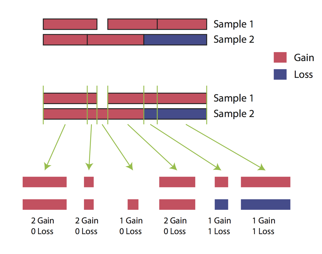
The cnFreq() function is much faster when all copy number segments have the same coordinates across all samples however this condition is not a requirement to run cnFreq(). It is important to talk about why and what goes on behind the scenes when this condition is not met as it may affect how we interpret the results. When segment coordinates are not identical cnFreq() will perform a disjoin operation and attempt to split segment coorinates so that they are identical across samples populating each coordinate with the appropriate copy number call. This is best illustrated in the two sample figure below. This operation may come with a loss of accuracy however as copy number calls are ussually made using the mean of many calls within that segment and splitting these segment up can therefore alter what the mean value of the copy number call would have been.
highlighting plot regions
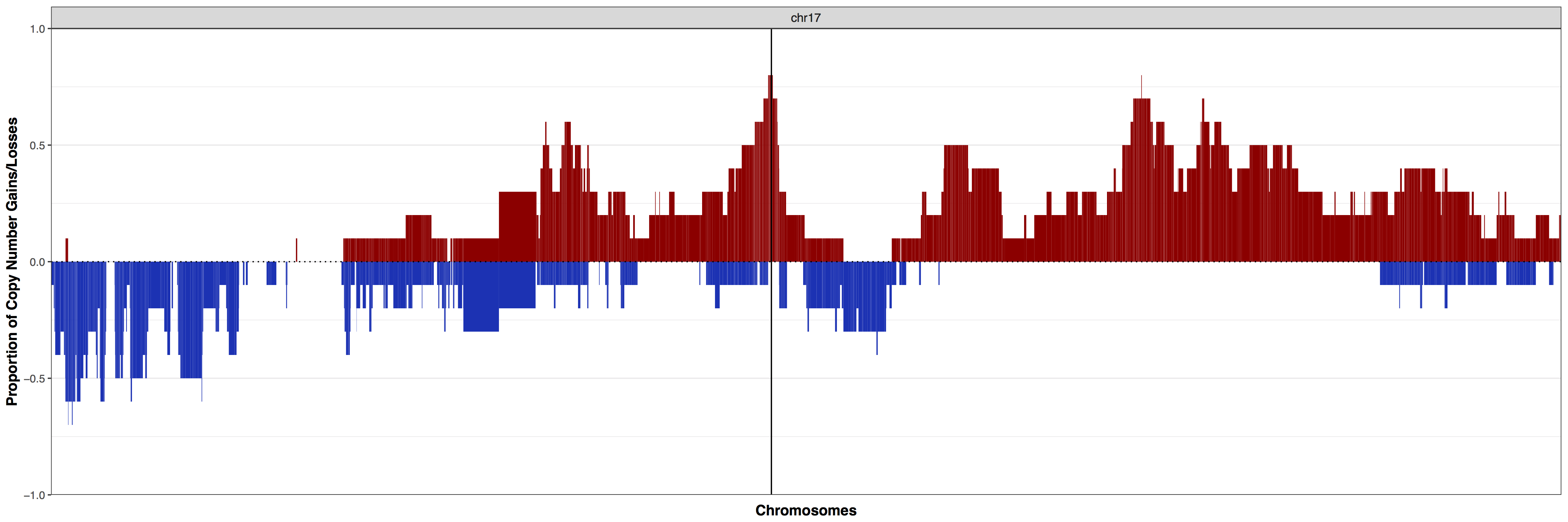
Let’s go back to our initial plot, what if we wanted to view a specific region of the genome such as ERBB2 (chr17:39,687,914-39,730,426) as these are HER2+ breast cancers. the function cnFreq() has the ability to zoom into specific chromosomes with the parameter plotChr and we have the ability to add additional layers onto our plot with the parameter plotLayer. Let’s go ahead and view just chromosome 17 and add in a vertical line where ERBB2 resides. As expected our vertical line intersects at a region where over 75% of samples are amplified. We can verify this by outputing the actual data calculations instead of the plot with the parameter out="data".
# highlight ERBB2
library(ggplot2)
layer1 <- geom_vline(xintercept=c(39709170))
cnFreq(cnData, genome="hg19", plotChr="chr17", plotLayer=layer1)
Exercises
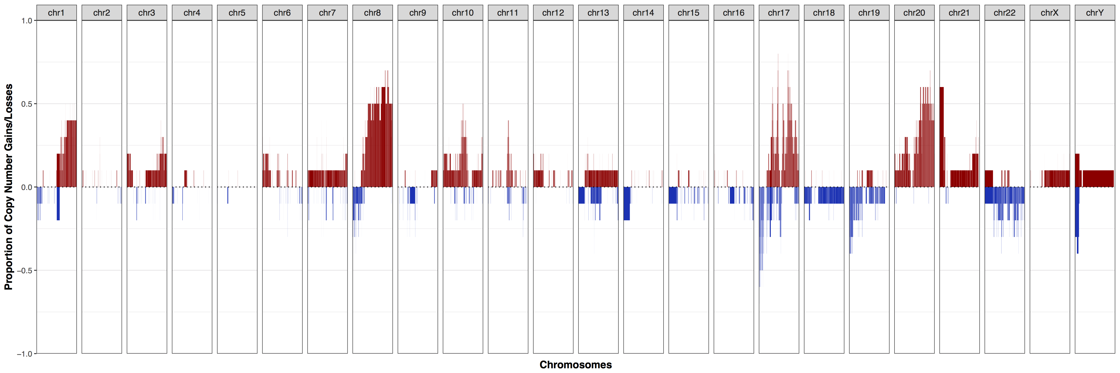
In almost all GenVisR functions the data frames which are used to produce plots can be extracted using the parameter out=data. This feature is not only usefull for looking at specific data values but also for infering what ggplot2 function calls or happening within GenVisR behind the scenes. With a bit of knowledge regarding ggplot2 we can overwrite core plot layers to do something specific. In the plots above we can tell that the function facet_grid() is being called just from looking at the plot. We can also see that facet_grid() is setting scales for each facet based on the size of each chromosome. Try overwriting this layer to remove this behavior with the parameter plotLayer. Your plot should look something like the one below.
Get a hint!
The parameter you will need to alter in facet_grid() is "scales="
Answer
facet_grid(. ~ chromosome, scales="free")
